Working with data in a data frame

As we saw earlier, read.csv loads tabular data from a CSV file into a data frame.

diabetes <- read.csv("r-intro-files/diabetes.csv")

class(diabetes)

## [1] "data.frame"

typeof(diabetes)

## [1] "list"

head(diabetes)

##   subject glyhb   location age gender height weight  frame
## 1   S1002  4.64 Buckingham  58 female     61    256  large
## 2   S1003  4.63 Buckingham  67   male     67    119  large
## 3   S1005  7.72 Buckingham  64   male     68    183 medium
## 4   S1008  4.81 Buckingham  34   male     71    190  large
## 5   S1011  4.84 Buckingham  30   male     69    191 medium
## 6   S1015  3.94 Buckingham  37   male     59    170 medium

colnames(diabetes)

## [1] "subject"  "glyhb"    "location" "age"      "gender"   "height"  
## [7] "weight"   "frame"

ncol(diabetes)

## [1] 8

nrow(diabetes)

## [1] 354

Indexing data frames

As with a matrix, a data frame can be accessed by row and column with [,].

One difference is that if we try to get a single row of the data frame, we get back a data frame with one row, rather than a vector. This is because the row may contain data of different types, and a vector can only hold elements of all the same type.

Internally, a data frame is a list of column vectors. We can use the $ syntax we saw with lists to access columns by name.

Logical indexing

A method of indexing that we haven’t discussed yet is logical indexing. Instead of specifying the row number or numbers that we want, we can give a logical vector which is TRUE for the rows we want and FALSE otherwise. This can also be used with vectors and matrices.

Suppose we want to look at all the subjects 80 years of age or over. We first make a logical vector:

is_over_80 <- diabetes$age >= 80

head(is_over_80)

## [1] FALSE FALSE FALSE FALSE FALSE FALSE

sum(is_over_80)

## [1] 9

>= is a comparison operator meaning greater than or equal to. We can then grab just these rows of the data frame where is_over_80 is TRUE.

diabetes[is_over_80,]

##     subject glyhb   location age gender height weight  frame
## 45    S2770  4.98 Buckingham  92 female     62    217  large
## 56    S2794  8.40 Buckingham  91 female     61    127   <NA>
## 90    S4803  5.71     Louisa  83 female     59    125 medium
## 130  S13500  5.60     Louisa  82   male     66    163   <NA>
## 139  S15013  4.57     Louisa  81 female     64    158 medium
## 193  S15815  4.92 Buckingham  82 female     63    170 medium
## 321  S40784 10.07     Louisa  84 female     60    192  small
## 323  S40786  6.48     Louisa  80   male     71    212 medium
## 324  S40789 11.18     Louisa  80 female     62    162  small

We might also want to know which rows our logical vector is TRUE for. This is achieved with the which function. The result of this can also be used to index the data frame.

which_over_80 <- which(is_over_80)
which_over_80

## [1]  45  56  90 130 139 193 321 323 324

diabetes[which_over_80,]

##     subject glyhb   location age gender height weight  frame
## 45    S2770  4.98 Buckingham  92 female     62    217  large
## 56    S2794  8.40 Buckingham  91 female     61    127   <NA>
## 90    S4803  5.71     Louisa  83 female     59    125 medium
## 130  S13500  5.60     Louisa  82   male     66    163   <NA>
## 139  S15013  4.57     Louisa  81 female     64    158 medium
## 193  S15815  4.92 Buckingham  82 female     63    170 medium
## 321  S40784 10.07     Louisa  84 female     60    192  small
## 323  S40786  6.48     Louisa  80   male     71    212 medium
## 324  S40789 11.18     Louisa  80 female     62    162  small

Comparison operators available are:

• x == y – “equal to”
• x != y – “not equal to”
• x < y – “less than”
• x > y – “greater than”
• x <= y – “less than or equal to”
• x >= y – “greater than or equal to”

More complicated conditions can be constructed using logical operators:

• a & b – “and”, true only if both a and b are true.
• a | b – “or”, true if either a or b or both are true.
• ! a – “not” , true if a is false, and false if a is true.

is_over_80_and_female <- is_over_80 & diabetes$gender == "female"

is_not_from_buckingham <- !(diabetes$location == "Buckingham")
# or
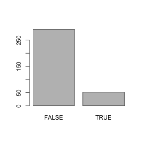
is_not_from_buckingham <- diabetes$location != "Buckingham"

The data we are working with is derived from a dataset called diabetes in the faraway package. The rows are people interviewed as part of a study of diabetes prevalence. The column glyhb is a measurement of percent glycated haemoglobin, which gives information about long term glucose levels in blood. Values of 7% or greater are usually taken as a positive diagnosis of diabetes. Let’s add this as a column.

diabetes$diabetic <- diabetes$glyhb >= 7.0

head(diabetes)

##   subject glyhb   location age gender height weight  frame diabetic
## 1   S1002  4.64 Buckingham  58 female     61    256  large    FALSE
## 2   S1003  4.63 Buckingham  67   male     67    119  large    FALSE
## 3   S1005  7.72 Buckingham  64   male     68    183 medium     TRUE
## 4   S1008  4.81 Buckingham  34   male     71    190  large    FALSE
## 5   S1011  4.84 Buckingham  30   male     69    191 medium    FALSE
## 6   S1015  3.94 Buckingham  37   male     59    170 medium    FALSE

Different ways to do the same thing

Above where we retrieved people 80 or over we could just as well have written:

weedle<- diabetes $age>=   80
diabetes[    weedle ,]

R does not understand or care about the names we give to variables, and it doesn’t care about spaces between things.

We could also have written it as a single line:

diabetes[diabetes$age >= 80,]

We can almost always unpack complex expressions into a series of simpler variable assignments. The naming of variables and how far to unpack complex expressions is a matter of good taste. Will you understand it when you come back to it in a year? Will someone else understand your code?

Missing data

summary gives an overview of a data frame.

summary(diabetes)

##     subject        glyhb              location        age       
##  S10000 :  1   Min.   : 2.680   Buckingham:178   Min.   :19.00  
##  S10001 :  1   1st Qu.: 4.385   Louisa    :176   1st Qu.:35.00  
##  S10016 :  1   Median : 4.840                    Median :45.00  
##  S1002  :  1   Mean   : 5.580                    Mean   :46.91  
##  S10020 :  1   3rd Qu.: 5.565                    3rd Qu.:60.00  
##  S1003  :  1   Max.   :16.110                    Max.   :92.00  
##  (Other):348   NA's   :11                                       
##     gender        height          weight         frame      diabetic      
##  female:206   Min.   :52.00   Min.   : 99.0   large : 91   Mode :logical  
##  male  :148   1st Qu.:63.00   1st Qu.:150.0   medium:155   FALSE:291      
##               Median :66.00   Median :171.0   small : 96   TRUE :52       
##               Mean   :65.93   Mean   :176.2   NA's  : 12   NA's :11       
##               3rd Qu.:69.00   3rd Qu.:198.0                               
##               Max.   :76.00   Max.   :325.0                               
##               NA's   :5       NA's   :1

We see that some columns contain NAs. NA is R’s way of indicating missing data. Missing data is important in statistics, so R is careful with its treatment of this. If we try to calculate with an NA the result will be NA.

1 + NA

## [1] NA

mean(diabetes$glyhb)

## [1] NA

Many summary functions, such as mean, have a flag to say ignore NA values.

mean(diabetes$glyhb, na.rm=TRUE)

## [1] 5.580292

There is also an is.na function, allowing us to find which values are NA, and na.omit which removes NAs.

not_missing <- !is.na(diabetes$glyhb)
mean( diabetes$glyhb[not_missing] )

## [1] 5.580292

mean( na.omit(diabetes$glyhb) )

## [1] 5.580292

na.omit can also be used on a whole data frame, and removes rows with NA in any column.

Factors

When R loads a CSV file, it tries to give appropriate types to the columns. Let’s examine what types R has given our data.

str(diabetes)

## 'data.frame':    354 obs. of  9 variables:
##  $ subject : Factor w/ 354 levels "S10000","S10001",..: 4 6 7 8 9 10 11 12 13 14 ...
##  $ glyhb   : num  4.64 4.63 7.72 4.81 4.84 ...
##  $ location: Factor w/ 2 levels "Buckingham","Louisa": 1 1 1 1 1 1 1 1 2 2 ...
##  $ age     : int  58 67 64 34 30 37 45 55 60 38 ...
##  $ gender  : Factor w/ 2 levels "female","male": 1 2 2 2 2 2 2 1 1 1 ...
##  $ height  : int  61 67 68 71 69 59 69 63 65 58 ...
##  $ weight  : int  256 119 183 190 191 170 166 202 156 195 ...
##  $ frame   : Factor w/ 3 levels "large","medium",..: 1 1 2 1 2 2 1 3 2 2 ...
##  $ diabetic: logi  FALSE FALSE TRUE FALSE FALSE FALSE ...

We might have expected the text columns to be the “character” data type, but they are instead “factor”s.

head( diabetes$frame )

## [1] large  large  medium large  medium medium
## Levels: large medium small

R uses the factor data type to store a vector of categorical data. The different possible categories are called “levels”.

Factors can be created from character vectors with factor. We sometimes care what order the levels are in, since this can affect how data is plotted or tabulated by various functions. If there is some sort of baseline level, such as “wildtype strain” or “no treatment”, it is usually given first. factor has an argument levels= to specify the desired order of levels.

Factors can be converted back to a character vector with as.character.

When R loaded our data, it chose levels in alphabetical order. Let’s adjust that for the column diabetes$frame.

diabetes$frame <- factor(diabetes$frame, levels=c("small","medium","large"))

head( diabetes$frame )

## [1] large  large  medium large  medium medium
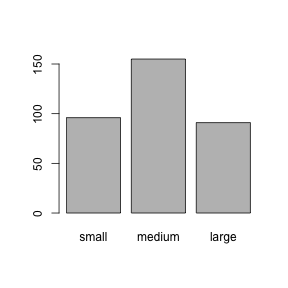
## Levels: small medium large

Plotting factors

Some functions in R do different things if you give them different types of argument. summary and plot are examples of such functions.

If we plot factors, R shows the proportions of each level in the factor. We can also see that R uses the order of levels we gave it in the plot.

plot( diabetes$frame )

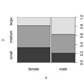
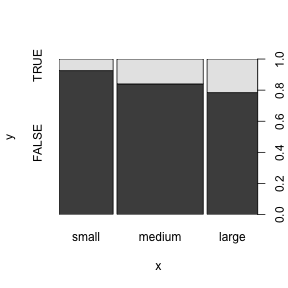
When we give R two factors to plot it produces a “mosaic plot” that helps us see if there is any relationship between the two factors.

plot( diabetes$gender, diabetes$frame )

diabetes$diabetic is logical, but we can tell R to turn it into a factor to produce this type of plot for this column as well.

plot( factor(diabetes$diabetic) )

plot( diabetes$frame, factor(diabetes$diabetic) )

Summarizing factors

The table function gives us the actual numbers behind the graphical summaries we just plotted (a “contingency table”).

table(diabetes$frame)

## 
##  small medium  large 
##     96    155     91

table(diabetes$diabetic, diabetes$frame)

##        
##         small medium large
##   FALSE    87    126    69
##   TRUE      7     24    19

Fisher’s Exact Test (fisher.test) or a chi-squared test (chisq.test) can be used to show that two factors are not independent.

fisher.test( table(diabetes$diabetic, diabetes$frame) )

## 
##  Fisher's Exact Test for Count Data
## 
## data:  table(diabetes$diabetic, diabetes$frame)
## p-value = 0.02069
## alternative hypothesis: two.sided

Summarizing data frames

We were able to summarize the dimensions (rows or columns) of a matrix with apply. In a data frame instead of summarizing along different dimensions, we can summarize with respect to different factor columns.

We already saw how to count different levels in a factor with table.

We can use summary functions such as mean with a function called tapply, which works similarly to apply. The three arguments we need are very similar to the three arguments we used with apply:

1. The data to summarize.
2. What we want not to be collapsed away in the output.
3. The function to use to summarize the data.

However rather than specifying a dimension for argument 2 we specify a factor.

tapply(diabetes$glyhb, diabetes$frame, mean)

##  small medium  large 
##     NA     NA     NA

We obtain NAs because our data contains NAs. We need to tell mean to ignore these. Additional arguments to tapply are passed to the function given, here mean, so we can tell mean to ignore NA with

tapply(diabetes$glyhb, diabetes$frame, mean, na.rm=TRUE)

##    small   medium    large 
## 4.971064 5.721333 6.035795

The result is a vector, with names from the classifying factor. These means of a continuous measurement seem to be bearing out our earlier observation using a discrete form of the measurement, that this data show some link between body frame and diabetes prevalence.

We can summarize over several factors, in which case they must be given as a list. Two factors produces a matrix. More factors would produce a higher dimensional array.

tapply(diabetes$glyhb, list(diabetes$frame, diabetes$gender), mean, na.rm=TRUE)

##          female     male
## small  5.042308 4.811379
## medium 5.490106 6.109464
## large  6.196286 5.929811

This is similar to a “pivot table”, which you may have used in a spreadsheet.

Melting a matrix into a data frame

You may be starting to see that the idea of a matrix and the idea of a data frame with some factor columns are interchangeable. Depending on what we are doing, we may shift between these two representations of the same data.

Modern R usage emphasizes use of data frames over matrices, as data frames are the more flexible representation. Everything we can represent with a matrix we can represent with a data frame, but not vice versa.

tapply took us from a data frame to a matrix. We can go the other way, from a matrix to a data frame, with the melt function in the package reshape2.

library(reshape2)

averages <- tapply(diabetes$glyhb, list(diabetes$frame, diabetes$gender), mean, na.rm=TRUE)
melt(averages)

##     Var1   Var2    value
## 1  small female 5.042308
## 2 medium female 5.490106
## 3  large female 6.196286
## 4  small   male 4.811379
## 5 medium   male 6.109464
## 6  large   male 5.929811

counts <- table(diabetes$frame, diabetes$gender)
melt(counts)

##     Var1   Var2 value
## 1  small female    66
## 2 medium female    96
## 3  large female    37
## 4  small   male    30
## 5 medium   male    59
## 6  large   male    54

Merging two data frames

One often wishes to merge data from two different sources. We want a new data frame with columns from both of the input data frames. This is also called a join operation.

Information about cholesterol levels for our diabetes study has been collected, and we have it in a second CSV file.

cholesterol <- read.csv("r-intro-files/chol.csv")
head(cholesterol)

##   subject chol
## 1   S1000  203
## 2   S1001  165
## 3   S1002  228
## 4   S1005  249
## 5   S1008  248
## 6   S1011  195

Great! We’ll just add this new column of data to our data frame.

diabetes2 <- diabetes
diabetes2$chol <- cholesterol$chol

## Error in `$<-.data.frame`(`*tmp*`, chol, value = c(203L, 165L, 228L, 249L, : replacement has 362 rows, data has 354

Oh. The two data frames don’t have exactly the same set of subjects. We should also have checked if they were even in the same order before blithely combining them. R has shown an error this time, but there are ways to mess up like this that would not show an error. How embarassing.

nrow(diabetes)

## [1] 354

nrow(cholesterol)

## [1] 362

length( intersect(diabetes$subject, cholesterol$subject) )

## [1] 320

Inner join using the merge function

We will have to do the best we can with the subjects that are present in both data frames (an “inner join”). The merge function lets us merge the data frames.

diabetes2 <- merge(diabetes, cholesterol, by="subject")

nrow(diabetes2)

## [1] 320

head(diabetes2)

##   subject glyhb   location age gender height weight  frame diabetic chol
## 1  S10001  4.01 Buckingham  21 female     65    169  large    FALSE  132
## 2  S10016  6.39 Buckingham  71 female     63    244  large    FALSE  228
## 3   S1002  4.64 Buckingham  58 female     61    256  large    FALSE  228
## 4  S10020  7.53 Buckingham  64   male     71    225  large     TRUE  181
## 5   S1005  7.72 Buckingham  64   male     68    183 medium     TRUE  249
## 6   S1008  4.81 Buckingham  34   male     71    190  large    FALSE  248

plot(diabetes2$chol, diabetes2$glyhb)

Note that the result is in a different order to the input. However it contains the correct rows.

Left join using the merge function

merge has various optional arguments that let us tweak how it operates. For example if we wanted to retain all rows from our first data frame we could specify all.x=TRUE. This is a “left join”.

diabetes3 <- merge(diabetes, cholesterol, by="subject", all.x=TRUE)

nrow(diabetes3)

## [1] 354

head(diabetes3)

##   subject glyhb   location age gender height weight frame diabetic chol
## 1  S10000  4.83 Buckingham  23   male     76    164 small    FALSE   NA
## 2  S10001  4.01 Buckingham  21 female     65    169 large    FALSE  132
## 3  S10016  6.39 Buckingham  71 female     63    244 large    FALSE  228
## 4   S1002  4.64 Buckingham  58 female     61    256 large    FALSE  228
## 5  S10020  7.53 Buckingham  64   male     71    225 large     TRUE  181
## 6   S1003  4.63 Buckingham  67   male     67    119 large    FALSE   NA

The data missing from the second data frame is indicated by NAs.

Appendix: Fitting models

A linear model tells you how various variables can be weighted together to predict an outcome. Many statistical tests can be thought of as comparing different linear models. Fitting linear models is well beyond the scope of this course, but we briefly mention them because this is one of the major uses of R.

mod1 <- lm(glyhb ~ age + frame + chol, data=diabetes2)
mod1

## 
## Call:
## lm(formula = glyhb ~ age + frame + chol, data = diabetes2)
## 
## Coefficients:
## (Intercept)          age  framemedium   framelarge         chol  
##     1.83635      0.04106      0.46343      0.55637      0.00716

summary(mod1)

## 
## Call:
## lm(formula = glyhb ~ age + frame + chol, data = diabetes2)
## 
## Residuals:
##     Min      1Q  Median      3Q     Max 
## -2.9964 -1.1943 -0.4479  0.2735  9.5144 
## 
## Coefficients:
##             Estimate Std. Error t value Pr(>|t|)    
## (Intercept) 1.836350   0.651191   2.820  0.00513 ** 
## age         0.041064   0.008041   5.107  5.9e-07 ***
## framemedium 0.463426   0.296694   1.562  0.11937    
## framelarge  0.556373   0.348871   1.595  0.11184    
## chol        0.007160   0.002983   2.400  0.01700 *  
## ---
## Signif. codes:  0 '***' 0.001 '**' 0.01 '*' 0.05 '.' 0.1 ' ' 1
## 
## Residual standard error: 2.138 on 294 degrees of freedom
##   (21 observations deleted due to missingness)
## Multiple R-squared:  0.1459, Adjusted R-squared:  0.1342 
## F-statistic: 12.55 on 4 and 294 DF,  p-value: 1.93e-09

We have obtained a model that, approximately

glyhb = 1.84 + 0.0411*age + 0.463*(frame=="medium") + 
        0.556*(frame=="large") + 0.00716*chol

There is considerable flexibility in the choice of variables which might be combined to predict the outcome. Perhaps frame is not informative if we already know age and chol, or perhaps other variables have predictive value. There are ways to test these questions statistically.

One problem here is that glyhb is skewed, and lm assumes errors in the model are normally distributed. A possible solution would be to try to fit a model to log(glyhb). Another possible solution is to try to model the binary outcome column diabetic instead, using logistic regression:

mod2 <- glm(diabetic ~ age + frame + chol, data=diabetes2, family="binomial")
summary(mod2)

## 
## Call:
## glm(formula = diabetic ~ age + frame + chol, family = "binomial", 
##     data = diabetes2)
## 
## Deviance Residuals: 
##     Min       1Q   Median       3Q      Max  
## -1.3242  -0.5763  -0.4013  -0.2351   2.6816  
## 
## Coefficients:
##              Estimate Std. Error z value Pr(>|z|)    
## (Intercept) -6.558692   1.113146  -5.892 3.81e-09 ***
## age          0.051632   0.011759   4.391 1.13e-05 ***
## framemedium  0.628803   0.483076   1.302   0.1930    
## framelarge   0.642442   0.518629   1.239   0.2154    
## chol         0.007699   0.003902   1.973   0.0485 *  
## ---
## Signif. codes:  0 '***' 0.001 '**' 0.01 '*' 0.05 '.' 0.1 ' ' 1
## 
## (Dispersion parameter for binomial family taken to be 1)
## 
##     Null deviance: 249.81  on 298  degrees of freedom
## Residual deviance: 215.68  on 294  degrees of freedom
##   (21 observations deleted due to missingness)
## AIC: 225.68
## 
## Number of Fisher Scoring iterations: 5

This model predicts the log odds of a patient having diabetes.

Again, this is well beyond the scope of this course. Just know that it is possible to construct a predictor of a continuous or binary outcome using R. Such predictors also tell you about the relative imporance of various explanatory variables. Consult a statistician if this approach is what you need.