6 QC Filtering
The steps below encompass the standard pre-processing workflow for scRNA-seq data in Seurat. These represent the selection and filtration of cells based on QC metrics, data normalization and scaling, and the detection of highly variable features.
6.1 QC and selecting cells for further analysis
Why do we need to do this?
Low quality cells can add noise to your results leading you to the wrong biological conclusions. Using only good quality cells helps you to avoid this. Reduce noise in the data by filtering out low quality cells such as dying or stressed cells (high mitochondrial expression) and cells with few features that can reflect empty droplets.
Seurat allows you to easily explore QC metrics and filter cells based on any user-defined criteria. A few QC metrics commonly used by the community include
- The number of unique genes detected in each cell.
- Low-quality cells or empty droplets will often have very few genes
- Cell doublets or multiplets may exhibit an aberrantly high gene count
- Similarly, the total number of molecules detected within a cell (correlates strongly with unique genes)
- The percentage of reads that map to the mitochondrial genome
- Low-quality / dying cells often exhibit extensive mitochondrial contamination
- We calculate mitochondrial QC metrics with the
PercentageFeatureSet()function, which calculates the percentage of counts originating from a set of features - We use the set of all genes starting with
MT-as a set of mitochondrial genes
# The $ operator can add columns to object metadata.
# This is a great place to stash QC stats
pbmc$percent.mt <- PercentageFeatureSet(pbmc, pattern = "^MT-")
Challenge: The meta.data slot in the Seurat object
Where are QC metrics stored in Seurat?
- The number of unique genes and total molecules are automatically calculated during
CreateSeuratObject()- You can find them stored in the object meta data
What do you notice has changed within the
meta.datatable now that we have calculated mitochondrial gene proportion?Imagine that this is the first of several samples in our experiment. Add a
samplenamecolumn to to themeta.datatable.
In the example below, we visualize QC metrics, and use these to filter cells.
- We filter cells that have unique feature counts over 2,500 or less than 200
- We filter cells that have >5% mitochondrial counts
#Visualize QC metrics as a violin plot
VlnPlot(pbmc, features = c("nFeature_RNA", "nCount_RNA", "percent.mt"), ncol = 3)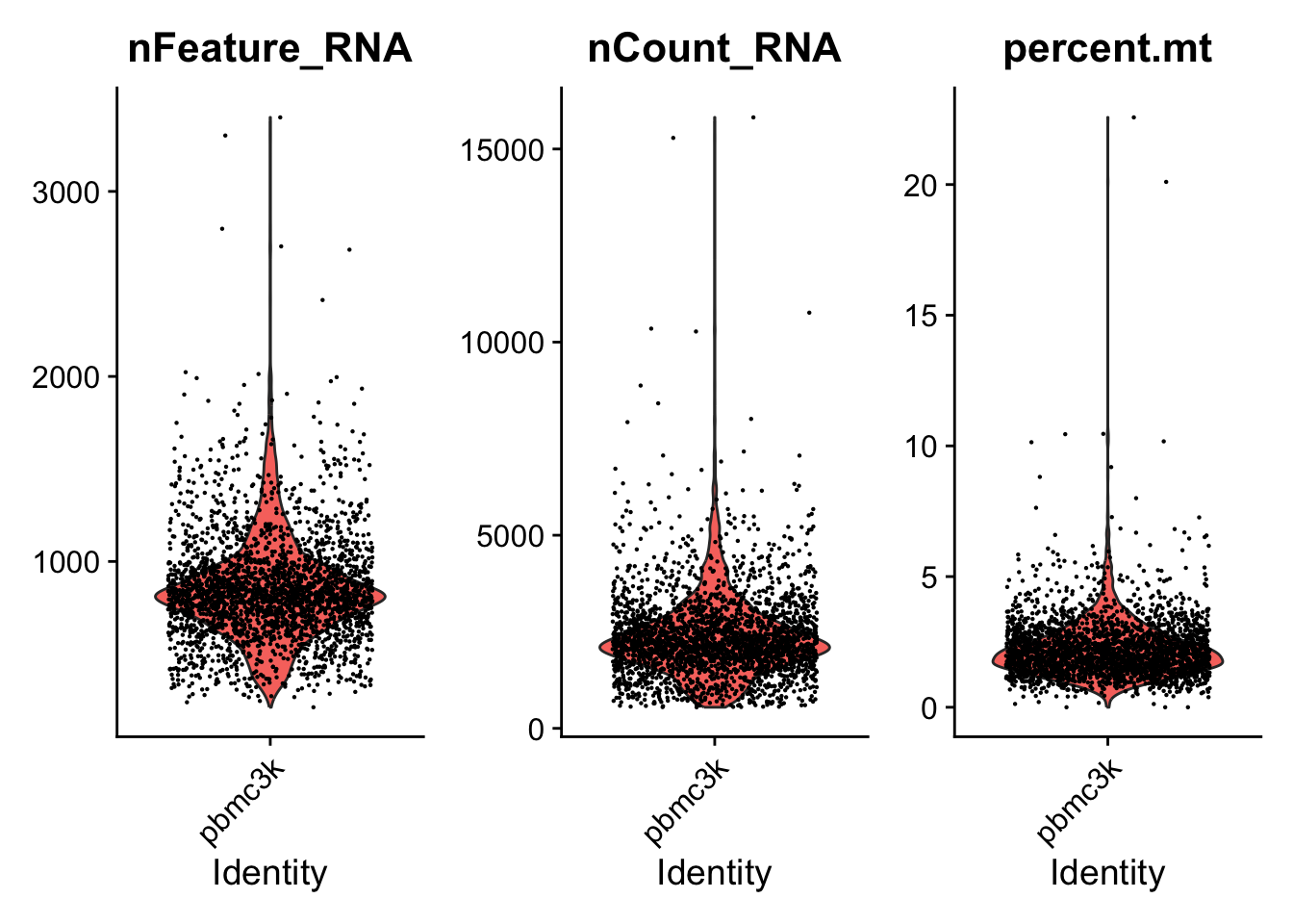
# visualize the max and min
VlnPlot(pbmc, features = "nFeature_RNA")+ scale_y_continuous(limits = c(1000,3000))
#> Scale for y is already present.
#> Adding another scale for y, which will replace the existing
#> scale.
#> Warning: Removed 2172 rows containing non-finite values
#> (`stat_ydensity()`).
#> Warning: Removed 2172 rows containing missing values
#> (`geom_point()`).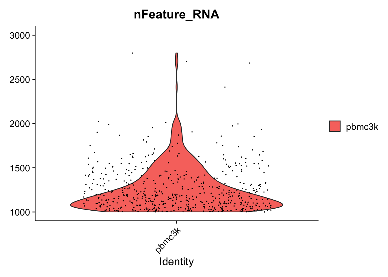
VlnPlot(pbmc, features = "nFeature_RNA",y.max =1000)
#> Warning: Removed 530 rows containing non-finite values
#> (`stat_ydensity()`).
#> Warning: Removed 530 rows containing missing values
#> (`geom_point()`).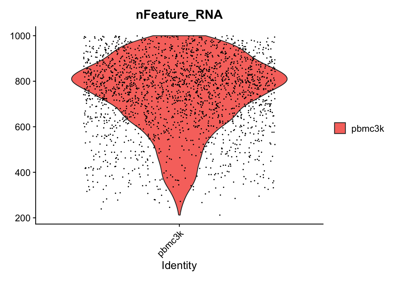
# FeatureScatter is typically used to visualize feature-feature relationships,
# but can be used for anything calculated by the object,
# i.e. columns in object metadata, PC scores etc.
plot1 <- FeatureScatter(pbmc, feature1 = "nCount_RNA", feature2 = "percent.mt")
plot2 <- FeatureScatter(pbmc, feature1 = "nCount_RNA", feature2 = "nFeature_RNA")
plot1 + plot2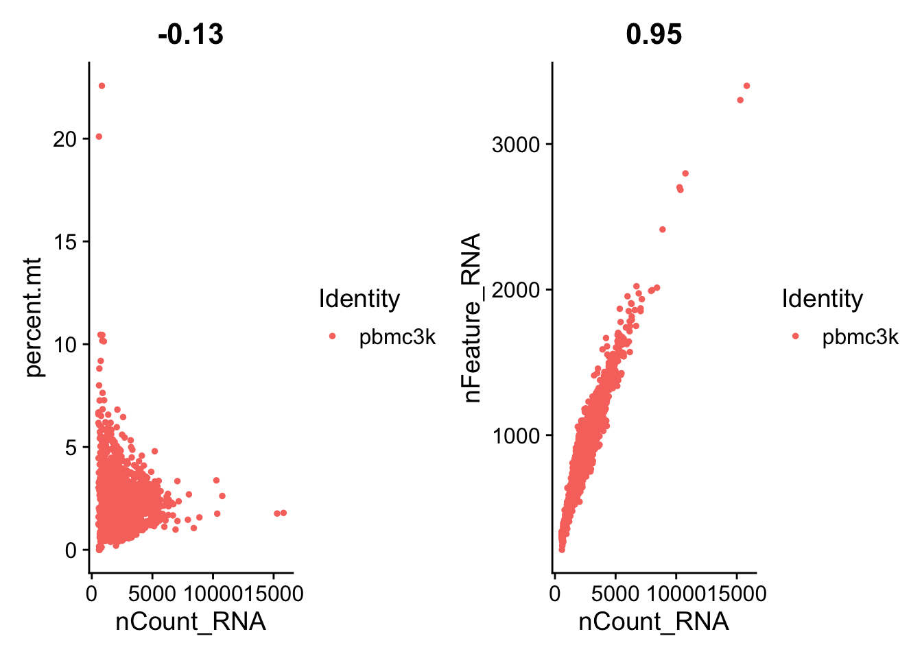
Lets look at the number of features (genes) to the percent mitochondrial genes plot.
plot3 <- FeatureScatter(pbmc, feature1 = "nFeature_RNA", feature2 = "percent.mt")
plot3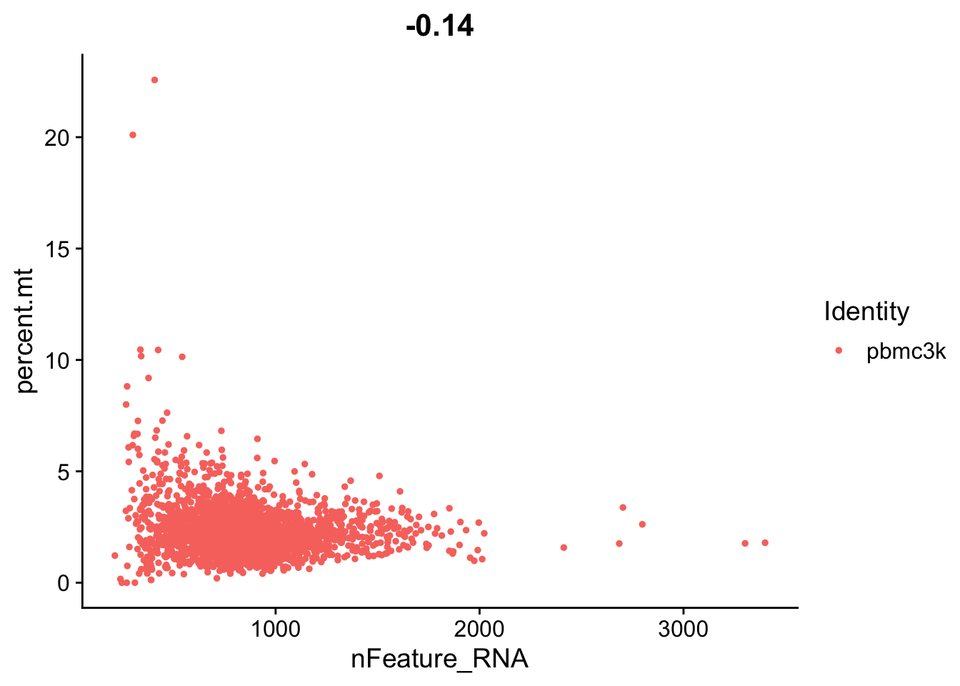
you can check different thresholds of mito percentage
#Number of cells left after filters
# percentage of cell with less than 10% mito
round(sum(pbmc$percent.mt < 10)/dim(pbmc)[2]*100,2)
#> [1] 99.78

# percentage of cell with less than 20% mito
round((sum(pbmc$percent.mt < 20)/dim(pbmc)[2])*100,2)
#> [1] 99.93

# percentage of cell with less than 30% mito
round((sum(pbmc$percent.mt < 30)/dim(pbmc)[2])*100,2)
#> [1] 100
Okay we are happy with our thresholds for mitochondrial percentage in cells, lets apply them and subset our data. This will remove the cells we think are of poor quality.
pbmc <- subset(pbmc, subset = nFeature_RNA > 200 & nFeature_RNA < 2500 & percent.mt < 5)Lets replot the feature scatters and see what they look like.
plot5 <- FeatureScatter(pbmc, feature1 = "nCount_RNA", feature2 = "percent.mt")
plot6 <- FeatureScatter(pbmc, feature1 = "nCount_RNA", feature2 = "nFeature_RNA")
plot5 + plot6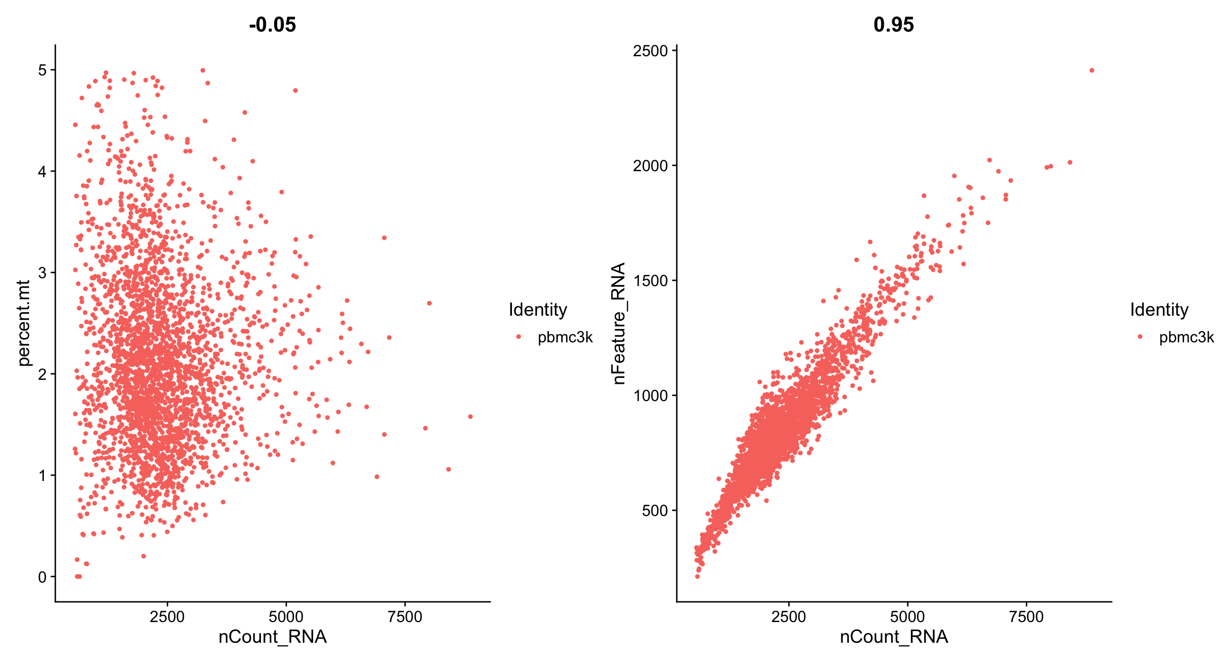
Challenge: Filter the cells
Apply the filtering thresolds defined above.
- How many cells survived filtering?
The PBMC3k dataset we’re working with in this tutorial is quite old. There are a number of other example datasets available from the 10X website, including this one - published in 2022, sequencing 10k PBMCs with a newer chemistry and counting method.
- What thresholds would you chose to apply to this modern dataset?