6 R Markdown

6.1 Introduction to markdown

Markdown is a powerful “language” for writing different kinds of documents, such as PDF or HTML in an efficient way, but markdown documents can also be published as is. The underlying idea for then markdown is that it is easy-to-write and easy-to-read.

You can use any text editor to write your markdown. RStudio already has an inbuilt text editor and because it also has a few additional things that make markdown writing much easier, we are going to use it’s text editor.

There are a few different flavours of markdown around. We’re going to mention a few but only focus on one, R Markdown

R markdown like most other flavours builds on top of standard markdown. It has some R language specific features as well as bunch of general enhancers to markdown. When R Markdown is coupled with Rstudio it creates a powerfull means of documenting your work while you are doing it, which you can then share with colleagues and the public in rapid and clean way.

Let’s get right into it. Firstly, if you haven’t installed it already, please install the rmarkdown package with:

install.packages("rmarkdown")

Open R Markdown file using these drop down menu steps: File -> New File -> R Markdown. You can put any title and any author name. For now select Document and Document type HTML. Once you have opened your .Rmd file, click on the Knit HTML button at the top of your pane.

Knitr is an R package that does all the magic of converting and running your R markdown and R code respectively. It’s installed when you install R Markdown.

These are three main parts to any R markdown document

YAML header section (will talk about it at the very end)

---
title: "Hello world"
author: "Kirill"
date: "13 July 2016"
output: html_document
---

The R code blocks section

 ```{r}
 plot(pressure)
 ```

Everything else is plain old markdown

# Have I been Marked Down

6.2 Document types

There are numerous document types that you can turn your markdown into. This all depends on the tool, markdown compiler, but for Rstudio at least these a few that a supported.

6.2.0.1 Documents

html_notebook - Interactive R Notebooks
html_document - HTML document w/ Bootstrap CSS
pdf_document - PDF document (via LaTeX template)
word_document - Microsoft Word document (docx)

6.2.0.2 Presentations (slides)

ioslides_presentation - HTML presentation with ioslides

6.2.0.3 More

tufte::tufte_handout - PDF handouts in the style of Edward Tufte
tufte::tufte_html - HTML handouts in the style of Edward Tufte
tufte::tufte_book - PDF books in the style of Edward Tufte

More here - including websites, books, etc

We are not going to cover all of them, we are mainly going to be working with either html_document or html_notebook both produce very similar results though behave slightly differently. We’ll try to touch a little on ioslides_presentation towards the end.

6.3 Vanilla Markdown

There’s actually not that much to core (vanilla) markdown. Essentially all of it can be summarised below:

# Header1
## Header2
### Header3

Paragraphs are separated
by a blank line.

Two spaces at the end of a line
produces a line break.  

Text attributes _italic_,
**bold**, `monospace`.

Horizontal rule:

---

Bullet list:

  * apples
  * oranges
  * pears

Numbered list:

  1. wash
  2. rinse
  3. repeat

A [link](http://example.com).

![Image](link_to_image)

> Markdown uses email-style
> characters for blockquoting.

Which produces:

Header1

Header2

Header3

Paragraphs are separated by a blank line.

Two spaces at the end of a line
produces a line break.

Text attributes italic, bold, monospace.

Horizontal rule:

Bullet list:

apples

oranges

pears

Numbered list:

wash

rinse

repeat

A link.

Markdown uses email-style > characters for blockquoting.

Whenever I need a refresher on markdown basics, I use this cheatsheet.

6.3.1 Practice vanilla markdown

Now it’s just a matter of learning some of the markdown syntax. Let’s delete all current text from the opened document except the YAML header and type this new text in Hello world, I'm learning R markdown! and pressing the Knit HTML button.

Hello world, I'm learning R markdown!

Not much happened. This is because we didn’t mark our text in any way. You can put as much text as you want and it will appear as is, unless “specially” marked to look differently.

Now add the # symbol at the start of the line and press the Knit HTML button again. We’ll be pressing this button a lot! For those who like keyboard short cuts use ctrl+shift+k instead.

# Hello world, I'm learning R markdown!

How about now? A single hash symbol made it whole lot bigger didn’t it? We’ve marked this whole line to be the header line.

Now make three new lines with the same text, but different numbers of # symbols, one, two and three respectively and keep pressing the Knit HTML button

### Hello world, I'm learning R markdown!
## Hello world, I'm learning R markdown!
# Hello world, I'm learning R markdown!

This is how you can specify different headers type using markdown.

Let’s now practice making very short document in markdown with a main topic section and two subsections. We will add short sentences in each section. We will start with main section header and a quote. Let’s type the following text and knit our document.

# Introduction

> Here, I'll talk about the rationale behind my experiment.

Now let’s add three bullet points summarising what we are going to write about in this document and knit the document again.

# Introduction

> Here, I'll talk about the rationale behind my experiment.

- Experimental Design
- Materials & Methods
- Analysis

Now let’s add each one of those bullet items as a subsection to the main “Introduction” section. We are going to use ## to mark subsections and don’t forget to knit again.

# Introduction

> Here, I'll talk about the rationale behind my experiment.

- Experimental Design
- Materials & Methods
- Analysis

## Experimental Design
## Materials & Methods
## Analysis

Now let’s add a sentence to each section, briefly describing what they are.

# Introduction

> Here, I'll talk about the rationale behind my experiment.

- Experimental Design
- Materials & Methods
- Analysis

## Experimental Design

> The organism used, number of samples I have, how many replicates, how many conditions.

## Materials & Methods

> What protocol I used, the reagents, the equipment.

## Analysis

> Once I got the raw data, how did I process & analyse it.

Let’s add a emphasis to some of the words in our document. We are going to add italic emphasis to the word “organism” and we are going to add bold emphasis to the capital letter “p” in the word protocol. You’ll need to knit your document still.

# Introduction

> Here, I'll talk about the rationale behind my experiment.

- Experimental Design
- Materials & Methods
- Analysis

## Experimental Design

The _organism_ used, number of samples I have, how many replicates, how many conditions.

## Materials & Methods

What **p**rotocol I used, the reagents, the equipment.

## Analysis

Once I got the raw data, how did I process & analyse it.

Remember that vanilla markdown is comprised entirely of punctuation characters.

6.4 Code Chunks

The reason that we are learning R Markdown is because it gives us a very straightforward way of writing plain text documents with inline R code that will become a very sophisticated document types. The bonus points also come from the fact that R Markdown files are easy to version control (git) and see the difference between versions.

This approach of interleaving analysis code, commentary and description is very explicit, which has direct implication in reproducibility, shareability and collaboration.

6.4.1 Embedding R code

An R chunk is a “special” block within the document that will be read and evaluated by knitr, ultimately converting everything into plain markdown. But for us it means that we can focus on our analysis and embed R code without having to worry about it. Additionally there are large number of chunk options that helps with different aspects of the document including code decoration and evaluation, results and plots rendering and display.

This is how an R code chunk looks like. If you want to include code into your documents it has to be via R chunks. You can further customise the appearance of your code in the final document with chunk options.

```{r}

```

The little r there specifies the “engine”, basically telling R Markdown how to evaluate the code inside the chunk. Here we are saying use R engine (language) to evaluate the code. The list of languages is rather long, R Markdown can span a much greater area then one might think. In this workshop we are only going to focus on R language.

Let’s write our first bit of R code inside the R Markdown document. First we need to start a new R chunk, which we can be done in these ways:

simply type it out
press insert button at the top of the window
ctrl+alt+i

Let’s return to our document with the sub header section Analysis. Now let’s add simple R code to our chunk, type the following code a <- "About to analyse my data!" and press knitr button to build html document. Note that as mentioned above we need to use print() statement to get the content of the variable to the scree/final document.

```{r}
a <- 'About to analyse my data!'
print(a)
```

Tip: each chunk can be run independently in the console by pressing ctrl^enter or little green arrow.

6.4.2 Chunk Options

We can tweak many things about your output using different options that we can include inside curly brackets e.g

```{r chunk_options, more_chunk_options...}

```

The two rather common options are echo=TRUE and eval=TRUE, both by default are set to true and this is why we didn’t have to pass them in previously.

echo means show what has been typed in i.e show the code in the final document
eval means evaluate or execute that code

Sometimes we might want to show the code, but not execute it and other times we might just want to execute it and get the results without actually bore audience with the code.

Let’s try both of these options one at a time. We start with passing echo=FALSE options first

 ```{r, echo = FALSE}
 print("About to analyse my data!")
 ```

Okay, we shouldn’t see our original print() statement in the output document. And now let’s pass eval=FALSE options instead

 ```{r eval = FALSE}
  print("About to analyse my data!")
 ```

And now we should only see the result of the print() statement and no output.

Here is a nice reference that has comprehensive cover of all the options you can pass in.

Let’s now try a different example and use the nuclear_xl_ms dataset from the proteomics viz segment for this next example. We’ll add another code chunk for it.

```{r}
library(tidyverse)
nuclear_xl_ms <- read_csv('r-intro-files/Nuclear_XL_MS.csv')
nuclear_xl_ms <- nuclear_xl_ms %>% mutate(
PPINovelty = factor(PPINovelty),
PPIEvidenceInfoGroup = factor(PPIEvidenceInfoGroup, levels = c('Structure','APID', 'STRING', 'Genetic', 'Unexplained'))
)
head(nuclear_xl_ms)
```

library(tidyverse)
nuclear_xl_ms <- read_csv('r-intro-files/Nuclear_XL_MS.csv')
nuclear_xl_ms <- nuclear_xl_ms %>% mutate(
  PPINovelty = factor(PPINovelty),
  PPIEvidenceInfoGroup = factor(PPIEvidenceInfoGroup, levels = c("Structure","APID", "STRING", "Genetic", "Unexplained"))
)
head(nuclear_xl_ms)

## # A tibble: 6 x 7
##   Protein1 Protein2 NameProtein1 NameProtein2 PPINovelty PPIEvidenceInfo…
##   <chr>    <chr>    <chr>        <chr>        <fct>      <fct>           
## 1 P02293   P04911   H2B1         H2A1         Known      Structure       
## 2 P02293   P02309   H2B1         H4           Known      Structure       
## 3 P02994   P32471   EF1A         EF1B         Known      Structure       
## 4 P0CX51   P38011   RS16A        GBLP         Known      Structure       
## 5 P02406   P0CX49   RL28         RL18A        Novel      STRING          
## 6 P33297   P53549   PRS6A        PRS10        Known      Structure       
## # … with 1 more variable: NumberUniqueLysLysContacts <dbl>

This table is a bit ugly to look at in your final document. We’ll come back to data-frame printing later in the YAML section.

Also examine the output carefully - you might notice that we’ve included the messages from library(tidyverse) and read_csv that are printed to the console by default. If you do not desire this behaviour and only want to see the output from head(nuclear_xl_ms) included in the document, message=FALSE is another code chunk option you can use.

6.4.3 Tip

You might be thinking that you’ve already run library(tidyverse) previously in the session and that you already have tidyverse packages loaded as well as read in and mutated the nuclear_xl_ms, you shouldn’t need to run these commands again. When you knit a document, it ignores the state of your RStudio session and runs through the code from start to finish. If your code points to missing files or uses packages that haven’t been explicitly loaded somewhere in the document, it will fail to render your document.

You can go between R Markdown and console, to check your code, at any time. You should see your code block is highlighted differently and you should see a green arrow at the right hand site of that block. Press the green arrow to get an output in the console. You can also use ctrl+enter to do the same with the keyboard short cut.

Here is a good example where we can hide our code from the viewer, since it isn’t most interesting bit about this data. Let’s turn echo=FALSE options for all our plots below.

Figure alignment can be done with fig.align options e.g {r fig.align=default} . default means what ever your style sheet has. The other options are, “left”, “center” and “right”. let’s try one out.

```{r, echo = FALSE, fig.align = 'right'}
ggplot(nuclear_xl_ms, aes(PPINovelty)) + 
geom_bar(aes(fill=PPIEvidenceInfoGroup)) + xlab('Novelty')
coord_flip() + theme_bw()
```

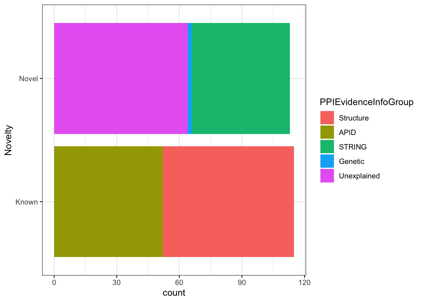
Remember that you can you always execute code in the console by pressing “green arrow” or using keyborad short cut ctrl+enter

We now know how to align figure to where we want, how about changing the size of it? We can do that with fig.height and fig.width, the units are inches. Let’s make 6 X 6 inches figure e.g {r fig.height=6, fig.width=6} . and also align the figure to the center

```{r, echo = FALSE, fig.align = 'right', fig.height=6, fig.width=6}
ggplot(nuclear_xl_ms, aes(PPINovelty)) + 
geom_bar(aes(fill=PPIEvidenceInfoGroup)) + xlab('Novelty')
coord_flip() + theme_bw()
```

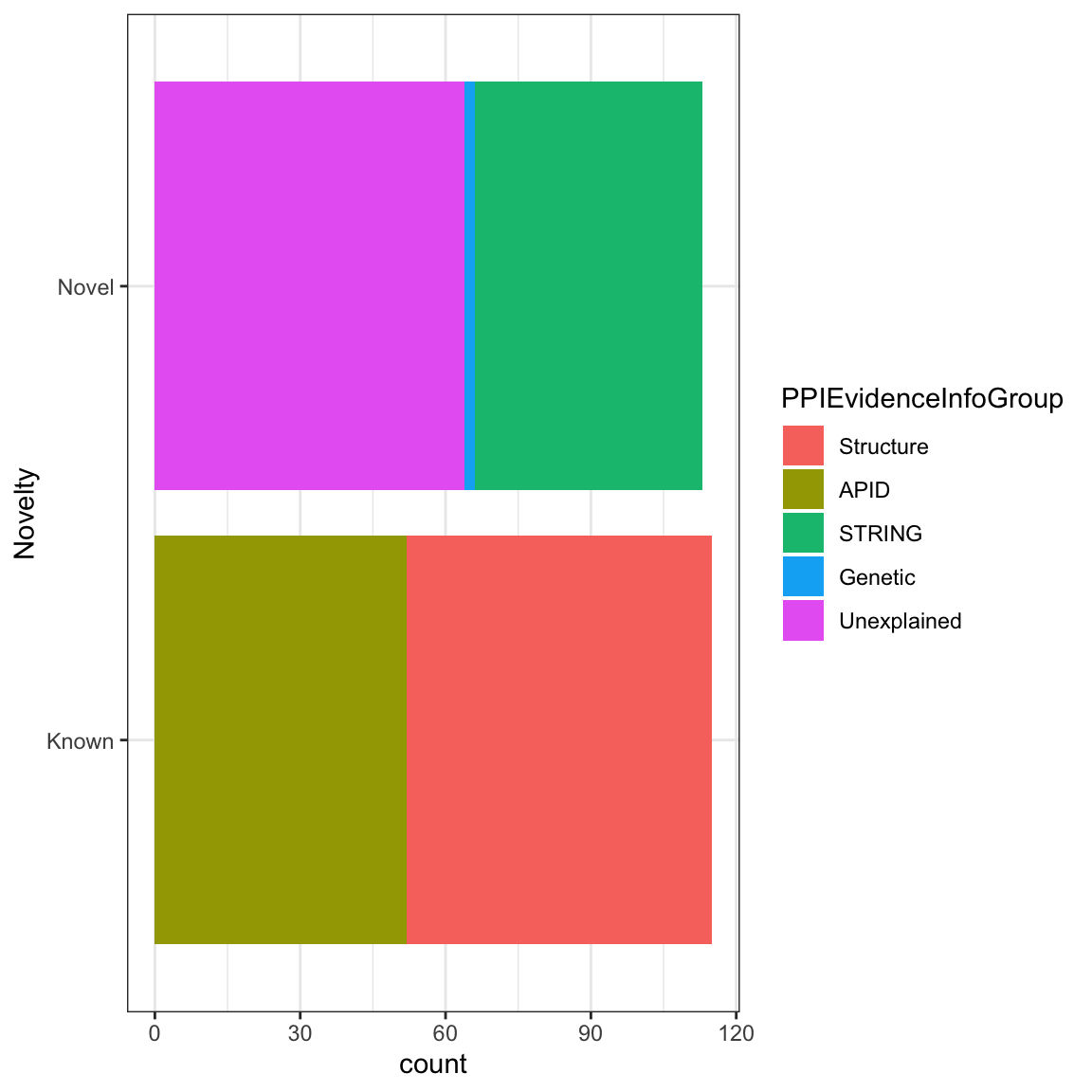
One last thing we’d like to share with you is how to add a figure legend or a caption - with fig.cap of course e.g {r, fig.cap="This is my legend"} . Go ahead and add a figure description.

```{r echo = FALSE, fig.align = 'center', warning=FALSE, fig.height=6, fig.width=6, fig.cap='This figure illustrates breakdown breakdown of protein-protein interaction evidence groups.'}
ggplot(gap_geo, aes(x=year, y=life_exp, group=name, color=region)) +
geom_line()
```

Figure 6.1: This figure illustrates breakdown breakdown of protein-protein interaction evidence groups.

Note that the figure legend follows the same alignment as the figure itself.

There are more chunk options which we encourage you to explore in greater depth in the R Markdown documentation. We have only examined a handful of figure specific options but there are many more options that allow fine control over the behavior of the code and cosmetics of the document.

Lastly, we’ll mention that the engine option can be used to specficy different language types. So you can embed python, BASH, Javascript and a heap of other languages all within the same document.

6.5 YAML header

At the very top of your .Rmd file you can, optionaly, include a YAML block. In this block you can fine turn your output document, add some metadata and change the document’s font and theme. You can also pass additional files such as stylesheet file .css and bibliography file .bib for text citation. We’re only going to show you a few possible options and will let you explore the rest on your own.

Navigate to the top of your .Rmd document and find the YAML section there. Just like with the options we passed in to manipulate R code block, YAML block also has key = value pairs, but instead they are separated by colon ( : ). Now let’s add table of content to our document, this will make it easier to navigate your page as well as give nice over view of the content our key is toc with value true or yes which one you prefer better.

 ---
 title: "Yeast Nuclear Protein interaction study"
 author: "Kirill"
 date: "13 July 2016"
 output:
   html_document:
     toc: true
 ---

Note that you need to bring html_document onto new line and indent it with two spaces. html_document is a value of output key. output can have other values e.g pdf_document, word_document. However html_document also becomes a key for toc value and toc becames a key for its own value.

Now that we have sort out the initial YAML layout, we can continue adding more options to style our HTML document. The other two useful options that I like to pass in are toc_depth and number_sections

---
title: "Yeast Nuclear Protein interaction study"
author: "Kirill"
date: "13 July 2016"
output:
  html_document:
    toc: true
    toc_depth: 4
    number_sections: yes
---

Most of those options are self explanatory. The best way to learn what each does, is to pass them in. Note that you can comment lines out inside YAML section with # symbol.

Another two options that can change your document apperance are theme and highlight. There are number of different themes and highlight options. I suggest you find the one you like in your own time.

Remember when we printed the nuclear_xl_ms data-frame, the table rendered wasn’t particularly nice to look at? We can control the behavior of tables in html documents in the YAML header. There are a number of options to select one from and pass to df_print.

Try out paged.

---
output:
  html_document:
    toc: true
    toc_depth: 4
    df_print: paged
---

6.6 Alternate Formats

As mentioned in a previous section, output has many options, one of which is ioslides_presentation. You can simple add:

---
title: "Hello world"
author: "Kirill"
date: "13 July 2016"
output: ioslides_presentation
---

at the top of your document and your .Rmd files will be compiled to a slide presentation instead.

Another way to start with an ioslides_presentation is select presentation options when you were opening R markdown file. Either way you’ll notice YAML header reflects your selected output type.

Let’s open new R markdown document and let’s select presentation instead and let’s select HTML (ioslides) option there. You can still save your files as .Rmd, and then press the the Knit HTML button.

The syntax for the document is more or less the same, except ## is now used to mark new slide.

ioslides are fairly basic in terms of slideshow presentations. If you find yourself frustrated with the limitations of ioslides, there are a number of official format options, we haven’t had much experience with using them. I’ve been using the xaringan package, which isn’t an official R Markdown format but I’ve found it to be quite powerful, though requires a fair degree of familiarity with R Markdown/HTMl/CSS.

Alternatively, if you want to produce a PDF document:

---
title: "Yeast Nuclear Protein interaction study"
author: "Kirill"
date: "13 July 2016"
output: pdf_document
---

R Markdown documents that render to PDF are compatible with raw LaTeX. The df_print option is not compatible with paged but will take kable and tibble. If changing document type, it’s always important to check which YAML options will carry to the new format and which won’t.

The more format specific syntax used in a document, the harder it is to swap a document from one format to another. For example, you can generate a very detailed and customised PDFs from an R Markdown document with heavy usage of LaTeX. However, LaTeX will not be rendered in a HTML document. So it’s important to have an idea of how the final document will be used as you work through it.

We’ve only just scratched the surface of what R Markdown can do! The online book we’ve been using throughout the course was written in R-Markdown and so were the slides for the workshop introduction.

6.7 More Resources

R Markdown cheatsheet

For a more in-depth R-Markdown tutorial, we recommend:

R Markdown: The Definitive Guide
bookdown: Authoring Books and Technical Documents with R Markdown - the bookdown package greatly extends R Markdown
R for Reproducible Research - a workshop delivered by the Monash Bioinformatics Platform focused on R Markdown and reproducible workflows with git.

6.7.1 Packages That Extend R-Markdown

blogdown - combines R Markdown & Hugo to create general purpose websites
bookdown - authoring books, thesis, sfotware manuals, etc
flexdashboards - HTML outputs with dashboard layouts
xaringan - slides shows with remark.js

6.7.2 Neat Examples:

Emi Tanaka’s personal website - blogdown for website, xaringan for slideshows, shiny + plotly for web apps
Rob Hyndman - another blogdown website. Also, see current top talk topic: How Rmarkdown changed my life - uses R Markdown for website, blog, text books, accademic papers, slides for talks, CV, thesis, exams, etc

6.7.3 Code chunk names

You can name code chunks! In your R-Studio session this even adds a little table of contents in the bottom left of your source panel that lets you navigate your R Markdown document via headers and code chunk names.

```{r chunk_name, chunk_opts...}

```

6.7.4 html_document or html_notebook

We’ve been using the html_document format for most of this tutorial. A very similar looking document is the html_notebook. There’s a large overlap in terms of YAML options for both.

e.g:

---
output:
  html_notebook:
    toc: true
    toc_depth: 4
    df_print: paged
---

One difference is that a html_notebook will include a button on the rendered webapge to download the .Rmd file that generated the html file. This is one way to easily share the document, in that someone can view your report and then download it and run it on their own machine.

The other difference is that when rendering a html_document, it will ignore the state of the RStudio session and re-run every code block. Variables that have been exist within the environment but have not been defined inside the html_document will cause the render step to fail and must be included for the document to render successfully.

A html_notebook however uses the state of the session. It will only include the output of code blocks that have been run. It’s less ‘safe’ using a notebook, because it doesn’t double-check that the document from start to finish is self-contained. It can include variables and functions that were created seperately in the environment but then the document doesn’t include instructions on how that variable was generated or what the function is doing.

6.7.5 Cross-referencing

Let’s learn how to add external and internal links to your document, remember the syntax for adding links is [DESCRIPTION](link-address). The external link that we are going to add is going to be this https://rmarkdown.rstudio.com/. Each one of the bullet points above going to become a link to it section. The way you reference internal section is by starting your address with a # symbol then simply using all lower case letters for the section name and all spaces need to be converted to a dash symbol -. Let’s add those things in and re-build our document.

# Learning Markdown

> I'm still learning

[External resource](https://rmarkdown.rstudio.com/)

Here I'll be learning:

- [markdown](#markdown)
- [R Markdown](#R Markdown)
- [git and github](#git-and-github)

## Markdown
Here I'll learning _vanilla_ markdown

## R Markdown

Whereas here I'll be learning **R**markdown

## ggplot2

And this section is about plotting

A bonus exercise is to add logos to each sections. Search internet for:

Markdown logo, and add the image using ![](link_address) syntax
R Markdown logo, and add the image using ![](link_address) syntax
Git logo, and add the image using ![](link_address) syntax
ggplot2 logo, and add the image using ![](link_address) syntax

Note for the external resource that is on internet the address must start with www or https otherwise address will be interpreted as file path.