Making sense of gene and proteins lists with functional enrichment analysis

17 Novel species FEA

FEA can be easily performed for many non-model species with user friendly web tools or R packages. g:Profiler web currently lists 1,113 supported organism records, and STRING currently (v12) supports 12,535 organisms.

Since many non-model species are supported by some FEA tools, today I am using the term novel species to describe a species that is not currently supported by any FEA tool.

Novel species FEA is possible with clusterProfiler or WebGestaltR in R, or using web tools WebGestalt or STRING. The requirements for each tool are slightly different, however at minimum a predicted proteome fasta is necessary. If you do not have a predicted proteome for your species, you would need to perform gene prediction, for which there are a number of in silico tools available. It must be kept in mind that in silico predicted proteomes can vary greatly in quality. Those that include multiple data sources such as polished genome assemblies generated with both short and long read shotgun sequencing and gene prediction that includes RNAseq data are likely to produce better gene predictions than those that are based only on for example short read sequencing.

Workflow overview of novel species annotation

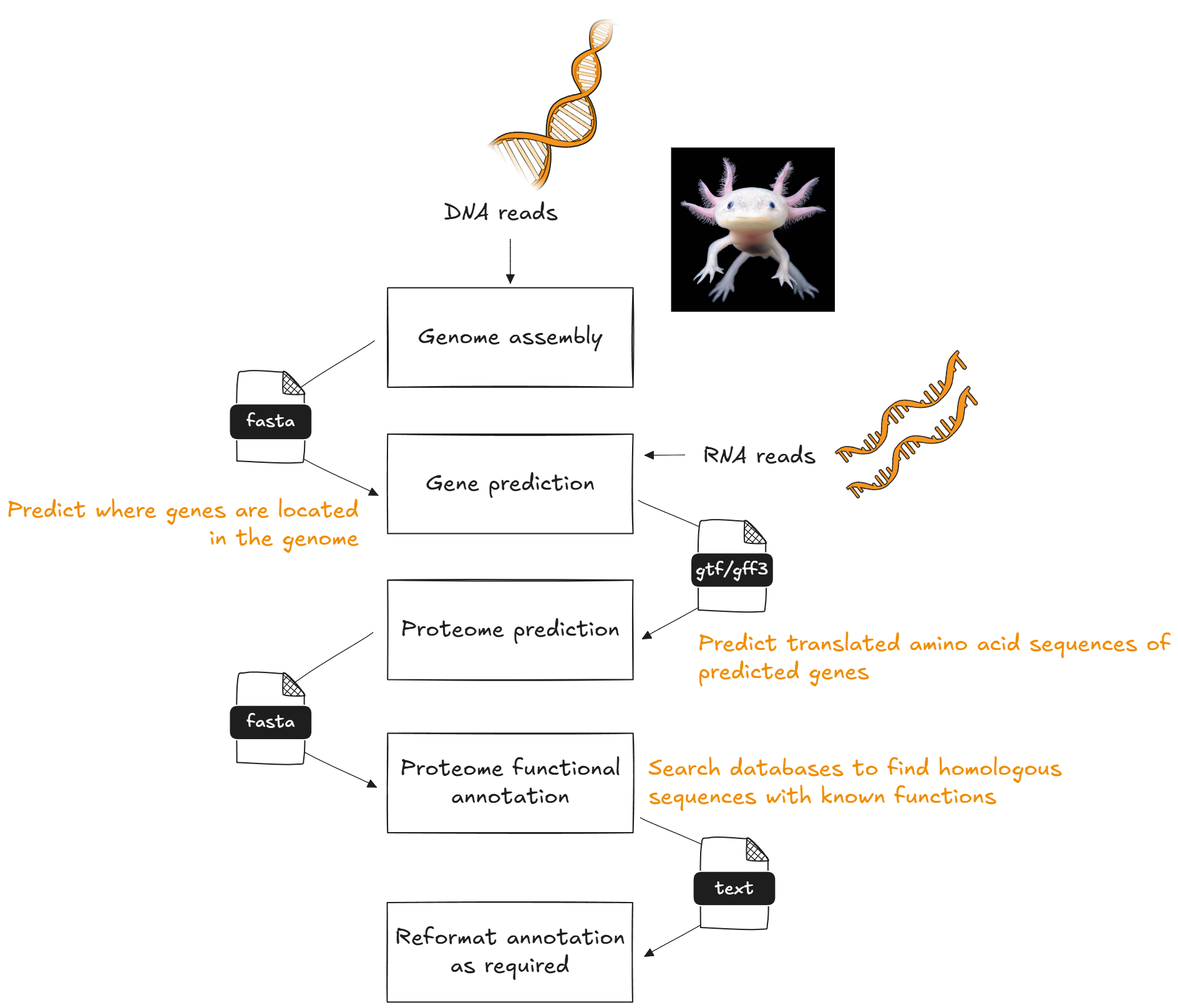
In this activity, we will use all three tools to perform FEA on a species that has a publicly available reference genome and gene predictions, but is not currently supported by any web-based FEA tool.

For clusterProfiler and WebGestaltR, we will import and reformat an annotation text file to match the requirements of the tools.

For STRING, we will use a STRING annotation on the web tool.

17.1 Axolotl functional enrichment analysis

17.1.1 Background

The axolotl (Ambystoma mexicanum) is a salamander with some very cool abilities: it can regenerate damaged or amputated tissue, including spinal cord and some brain regions. While this species has reference genome on NCBI, it is not annotated. There is no axolotl Org.db Bioconductor annotation package available nor does this species exist in KEGG Organisms. There is however an axolotl genome browser where you can download a (slightly less contiguous than the NCBI version) reference genome plus a (non-curated) GTF file.

Despite the lack of quality resources, there is much ’omics work conducted in axolotl due to its regenerative capabilities.

Today we will use public RNAseq data from axolotl, comparing gene expression in the blastema after proximal (at the shoulder) and distal (at the hand) limb amputation. The blastema is a collection of undifferentiated progenitor cells that give rise to the regenerated limb. Maybe our functional enrichment analysis of differentially expressed genes can help us understand processes that cause the blastema to grow into a full limb or just a hand!

17.1.2 Caveat!

This is not a real experiment! It was tricky to find a novel species that had:

a reference genome
a GTF
was not natively supported by any FEA tool
had publicly available RNAseq data
FEA described in a peer-reviewed study

This axolotl data ticked A through D yet not E (RNA from various tissues were sequenced to aid a genome assembly project rather than for a valid biological experiment). Please keep this in mind when reviewing the results of the FEA we perform 😉 The goal of the session is not really to uncover how a blastema differentiates into a hand or an arm, but to demonstrate to you how you can apply this method to your own novel species.

17.1.3 Raw data sources

17.1.4 Data preparation

17.1.4.1 Annotation files

The reference genome and GTF gene prediction file were downloaded from www.axolotl-omics.org. A proteome was created by extracting the predicted peptide sequences from the GTF then retaining the longest isoform per gene with AGAT v 1.4.0. The predicated proteome was then annotated with eggNOG emapper v 2.1.12.

The annotation output file has been provided to you, and we will import this into R and use the dplyr package v 1.1.4 to extract GO and KEGG IDs into the required format for R-based FEA with clusterProfiler and WebGestaltR.

The predicted proteome was also annotated with STRING v 12.0. As of version 12, STRING includes a feature Add any organism to STRING / Annotate proteome (Szklarczyk et al 2023). The axolotl proteome was uploaded to STRING and annotation performed on STRING servers in less than 1 day. The resulting annotation is persistent and shareable and can be used for all of STRING’s search functions including ORA (Multiple proteins) and GSEA (Proteins with Values/Ranks).

17.1.4.2 Reads processing and differential expression analysis

Broadly following https://github.com/Sydney-Informatics-Hub/RNASeq-DE, The raw RNAseq fastq were downloaded from Bioproject, quality trimmed and adapters removed with BBtools bbduk v 39.01, then aligned to the reference genome with STAR v 2.7.11b. Feature counting was performed with HTSeq-counts v 2.0.3 and formatted into a counts matrix. Differential gene expression analysis was performed in R with DESeq2 v 1.46.0, filtering for genes with at least a count of 10 in at least 2 samples. The data comprises 2 groups (proximal blastema and distal blastema) and 2 replicates per group.

The DE results file has been provided to you, and we will import this into R to extract our gene lists.

17.2 Activity overview

Import emapper axolotl annotation file, GO ontology file and KEGG Pathways file
Import axolotl DE results file and extract gene lists for ORA and GSEA
Reformat annotation files for clusterProfiler GO and KEGG analysis
Run clusterProfiler universal FEA functions enricher and GSEA and visualise results with enichPlot
Reformat annotation files for WebGestaltR GO and KEGG analysis
Run WebGestaltR ORA and GSEA and visualise results in the interactive HTML report
Run ORA with STRING online using custom axolotl annotation
Compare STRING ORA web results to those generated using the emapper annotations in R

Before heading over to RStudio, we will briefly review the annotation requirements for the R tools. At the end of the R-based analysis, we will return here for the web-based analysis with STRING.

17.3 R-based FEA

17.3.1 clusterProfiler

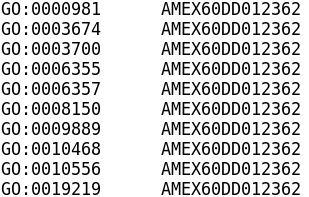
This tool can perform ORA or GSEA for any organism with the provision of custom TERM2GENE and TERM2NAME files. TERM2GENE maps the species gene ID to database (eg GO, KEGG) terms, and TERM2NAME maps the terms to their descriptive names. The gene IDs for our axolotl annotation are prefixed with AMEX60DD.

Example TERM2GENE format:

Example TERM2NAME format:

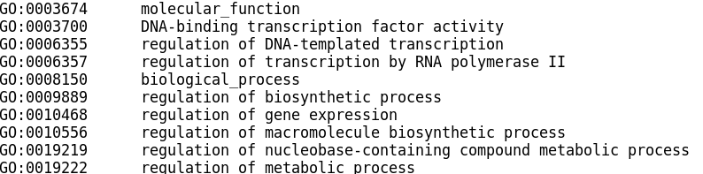
These are then provided to the universal enrichment functions GSEA and enricher (ORA). It is essential that the gene lists provided have the same gene IDs as those in the TERM2GENE file.

In RStudio, we will extract these file formats from the emapper annotations file for axolotl and proceed with FEA.

We are using GO and KEGG today, however you can use any database, provided you first annotate your proteome to the database in order to obtain the term to name mappings.

Acknowledgement to Armin Dadras for sharing his code to extract TERM2GENE and TERM2NAME from emapper output.

17.3.2 WebGestaltR

This tool can perform ORA or GSEA for any organism with the provision of custom GMT and description files.

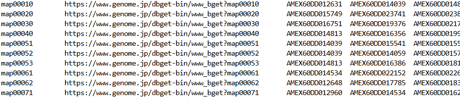
The GMT file format is slightly different than the typical gene set matrix transposed file format you may have seen before, which typically has the gene set description in the second column. For WebGestaltR, the description is in a separate file, and the tab-delimited GMT file with .gmt suffix has these 3 columns:

Gene set ID
Web link for gene set
Third and subsequent columns are genes belonging to the gene set

Example .gmt format:

The WebGestaltR tab delimited description file with .des suffix has these columns:

Gene set ID
Gene set description

Example .des format:

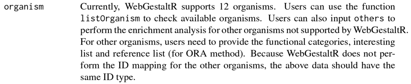
These files are then provided to the single FEA function within the package. The function has the same name as the package - WebGestaltR. Users control the analysis type by providing one of ORA, GSEA or NTA arguments to the parameter enrichMethod.

The .gmt file is provided to the parameter enrichDatabaseFile and the .des file is provided to the parameter enrichDatabaseDescriptionFile. Specifying organism = "others" is also required to run the FEA analysis with the custom databse files. It is essential that the .gmt file has the same gene IDs as those in query gene list.

17.3.3 Mapping database terms to descriptions

Annotating a proteome with a tool such as emapper provides a connection between your novel species gene IDs and term IDs. To add the term description, we need a database file. In this analysis, we will use the GO ‘core’ ontology file and the KEGG Pathways file. These files were downloaded to the workshop folder of the VMs during our setup session.

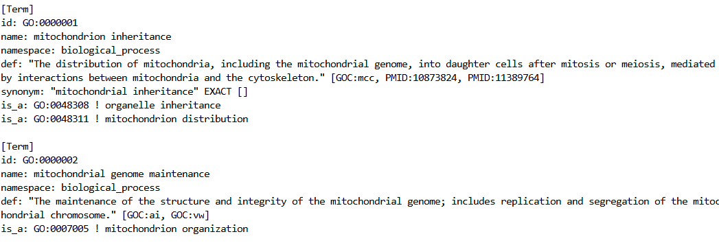
The GO go.obo is a text file (>600K lines) with details for all terms in GO at the time of download. The second line of the file contains the GO database version, in this case: data-version: releases/2024-06-17.

go.obo term information is structured like this:

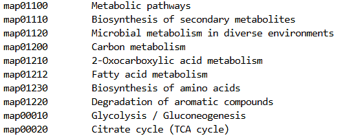
The KEGG Pathways file is identical in format to what is required for both the clusterProfiler TERM2NAME and WebGestaltR .des files:

KEGG Patwhays file format:

17.4 Analysis workflow

The complete executable analysis is included below. Run the code chunks interactively while working through the chapter, or render the full Bookdown project to execute the analysis and retain the code, parameters, results, figures, and software-version information in the book output.

library(readr)
library(dplyr)
library(ontologyIndex)
library(tidyverse)
#> ── Attaching core tidyverse packages ──────────────────────────────────────────── tidyverse 2.0.0 ──
#> ✔ forcats 1.0.1     ✔ stringr 1.6.0
#> ✔ purrr   1.2.2     ✔ tibble  3.3.1
#> ── Conflicts ────────────────────────────────────────────────────────────── tidyverse_conflicts() ──
#> ✖ IRanges::%within%()       masks lubridate::%within%()
#> ✖ IRanges::collapse()       masks dplyr::collapse()
#> ✖ Biobase::combine()        masks BiocGenerics::combine(), dplyr::combine()
#> ✖ IRanges::desc()           masks dplyr::desc()
#> ✖ S4Vectors::expand()       masks tidyr::expand()
#> ✖ clusterProfiler::filter() masks dplyr::filter(), stats::filter()
#> ✖ S4Vectors::first()        masks dplyr::first()
#> ✖ dplyr::group_rows()       masks kableExtra::group_rows()
#> ✖ dplyr::lag()              masks stats::lag()
#> ✖ BiocGenerics::Position()  masks ggplot2::Position(), base::Position()
#> ✖ purrr::reduce()           masks IRanges::reduce()
#> ✖ S4Vectors::rename()       masks clusterProfiler::rename(), dplyr::rename()
#> ✖ S4Vectors::second()       masks lubridate::second()
#> ✖ S4Vectors::second<-()     masks lubridate::second<-()
#> ✖ AnnotationDbi::select()   masks biomaRt::select(), clusterProfiler::select(), dplyr::select()
#> ✖ purrr::simplify()         masks clusterProfiler::simplify()
#> ✖ IRanges::slice()          masks clusterProfiler::slice(), dplyr::slice()
#> ℹ Use the conflicted package (<http://conflicted.r-lib.org/>) to force all conflicts to become errors
library(clusterProfiler)
library(WebGestaltR)
#> ******************************************
#> 
#> *                                        *
#> 
#> *          Welcome to WebGestaltR !      *
#> 
#> *                                        *
#> 
#> ******************************************
library(enrichplot)

17.5 Working directory

Ensure the ‘workshop’ directory is your current working directory. (“workshop” refers to your own RStudio project folder if you’re running this during the live session — the code below handles the book’s own relative paths automatically.)

# Bookdown evaluates relative file paths from the book project directory.
# Confirm the directory from which the book is being rendered.
getwd()
#> [1] "/home/runner/work/Functional_Enrichment_Web_and_Command_Line/Functional_Enrichment_Web_and_Command_Line"
# root.dir is a book-wide knitr option, not scoped to this chapter, so we
# save it here and restore it at the end of the chapter (see "Restore
# working directory" below) - otherwise every later chapter would inherit
# this chapter's working directory, breaking their relative file paths.
novel_species_book_root_dir <- getwd()
knitr::opts_knit$set(root.dir = "data/R_data")
getwd()
#> [1] "/home/runner/work/Functional_Enrichment_Web_and_Command_Line/Functional_Enrichment_Web_and_Command_Line"

17.6 Import `emapper` axolotl annotation file, GO ontology file and KEGG Pathways file

See Raw data sources and Data preparation above for the full data provenance and processing pipeline behind the files imported below.

17.6.1 Import annotation files

17.6.1.1 emapper proteome annotation

The emapper annotation output contains results against a number of databases including GO and KEGG, which we will focus on today.

eggnog_anno <- read_tsv("AmexG_v6.0-DD.emapper.annotations.txt", show_col_types = FALSE)
head(eggnog_anno)

The raw annotation file provides us with ‘term ID to gene ID’ mappings for our species. We also need ‘term ID to term description’ mappings. These files are not organisms specific: we will extract only the terms that are found within our custom species annotation, to make our organism specific version.

17.6.1.2 GO Core Ontology

For GO, we will use the GO ‘core’ ontology file, downloaded from https://purl.obolibrary.org/obo/go.obo and included in the data files you downloaded to workshop directory earlier.

We will use the ontologyIndex package to retrieve ontology info and save to an object named ontology for later use creating the required custom database files for clusterProfiler and WebGestaltR.

ontology <- ontologyIndex::get_ontology(
  file = "go.obo",
  propagate_relationships = "is_a", # propagates relationships from parent terms to children
  extract_tags = "everything", # retrieve all available details for each term
  merge_equivalent_terms = TRUE
) # avoid unecessary redundancy

17.6.1.3 KEGG Pathways

For KEGG, we have both map and ko IDs in our emapper annotation.

ko terms (https://www.genome.jp/kegg/ko.html) represent orthologous groups of genes, which are assigned based on evolutionary relationships and functional similarity, so can provide more precise functional categorisation which can be particularly useful when working with novel species which lack curate dpathway information.

map terms (https://www.genome.jp/kegg/pathway.html) are manually drawn pathway maps representing KEGG database of molecular interaction, reaction and relation networks for: Metabolism, Genetic Information Processing, Environmental Information Processing, Cellular Processes, Organismal Systems, Human Diseases, and Drug Development.

Today we will be working with the map terms due to database download restrictions.

Free access to the KEGG FTP downloads requires an academic subscription, to which you must confirm to be the “only user of the KEGG FTP Data”. The pathways list was available freely. As a single user, you can request academic access here https://www.pathway.jp/en/academic.html.

There is an alternate method for using ko IDs, which uses the KEGG ontology information available through the clusterProfiler functions enrichKEGG and gseKEGG. An example of the R code can be found here https://github.com/dadrasarmin/enrichment_analysis_for_non_model_organism. However, this poses a problem: as the novel species gene IDs are assigned to KEGG terms, gene:name duplicate records are identified, and duplicates must be removed in order to avoid errors running the enrichment. This loss of data will have a real impact on the results, with the importance of some terms being underestimated.

Given these considerations, we will proceed with map pathway terms :-)

The KEGG map pathway list was downloaded from https://rest.kegg.jp/list/pathway and downloaded to your workshop directory.

kegg_pathways <- read.table("kegg_pathways_2024-11-13.txt", header = FALSE, sep = "\t", col.names = c("term", "name"))
head(kegg_pathways)

17.7 Import axolotl DE results file and extract gene lists for ORA and GSEA

17.7.1 Import axolotl DE data

Load the DE results file for axolotl:

de_matrix <- read_tsv("axolotl_DE_results.txt", col_names = TRUE, show_col_types = FALSE)
head(de_matrix)

17.7.2 Create the ranked gene list for GSEA

Recall from the last 2 activities that clusterProfiler requires a vector object for GSEA, while WebGestaltR requires a 2-column dataframe. Since we intend to use both tools, let’s create both now:

# Create ranked vector for clusterProfiler GSEA
ranked_vector <- setNames(de_matrix$log2FoldChange, de_matrix$geneID) %>% sort(decreasing = TRUE) # Named vector

# check
head(ranked_vector)
tail(ranked_vector)

# Create ranked dataframe for WebGestaltR GSEA# extract ranked dataframe
ranked_df <- de_matrix %>%
  arrange(desc(log2FoldChange)) %>%
  dplyr::select(geneID, log2FoldChange)

# check
head(ranked_df)
tail(ranked_df)

17.7.3 Create gene lists for ORA

For ORA, both tools require vector class gene lists. We will filter for adjusted P value < 0.01 and absolute log2 fold change greater than 1.5.

The matrix has already filtered out genes with very low counts so we take all genes present as the background.

# Filter for DEGs and save gene IDs as vector
degs <- de_matrix %>%
  filter(padj <= 0.01 & abs(log2FoldChange) >= 1.5) %>%
  pull(geneID) # Extract

# Extract the background gene list vector
background <- de_matrix %>%
  pull(geneID)

# Check number of genes:
cat("Number of DEGs:", length(degs), "\n") # Number of DEGs
cat("Number of background genes:", length(background), "\n") # Number of background genes

# Check format:
head(degs)
head(background)

Note the large drop in gene numbers: 100K in GTF, 48K in predicted proteome, 24K expressed in the blastema! By reducing the number of background genes to what are expressed in the studied tissue, we can reduce falsely inflated P values and false positives within our list of enriched terms.

17.7.4 Save gene lists

Saving any outputs generated from R code is vital to reproducibility! You should include all analysed gene lists within the supplementary materials of your manuscript.

# Save DEGs
write.table(degs, file = "Axolotl_DEGs.txt", quote = FALSE, col.names = FALSE, row.names = FALSE, sep = "\t")
# Save background
write.table(background, file = "Axolotl_background.txt", quote = FALSE, col.names = FALSE, row.names = FALSE, sep = "\t")
# Save ranked
write.table(ranked_df, file = "Axolotl_rankedFC.txt", sep = "\t", quote = FALSE, row.names = FALSE, col.names = TRUE)

17.8 Reformat annotation files for `clusterProfiler` GO and KEGG analysis

Now we have annotation files and gene lists, we will bring those together to create the custom database files required for R FEA!

17.8.1 Create TERM2GENE files

These are 2 column text files with the term ID (one per line) alongside the ID of the gene that maps to the term. A gene can map to many terms and thus be present on multiple lines. A term can be mapped to more than one gene and thus be present on many lines.

Check the column names of the emapper annotation file so we know which are the GO and KEGG column names:

colnames(eggnog_anno)

We need GOs and KEGG_Pathway columns.

17.8.1.1 GO TERM2GENE

Next, we will extract the GO IDs from the emapper annotation file, and wrangle into the correct format for clusterProfiler TERM2GENE.

There are several steps to this - comments have been included to outline what each step is doing.

go_term2gene <- eggnog_anno %>%
  dplyr::select(GOs, `#query`) %>% # select the GO column and the query column (axolotl gene ID)
  dplyr::filter(GOs != "-") %>% # filter out rows where the GO ID is "-" ie no GO annotation for this gene
  separate_rows(GOs, sep = ",") %>% # split comma-delimited list of many GO terms for a gene into separate rows
  dplyr::select(GOs, `#query`) %>% # keep the GO and query columns
  distinct() %>% # remove any duplicate rows
  drop_na() # remove rows with missing values

# Rename columns to match desired output format
colnames(go_term2gene) <- c("term", "gene")

# Save to file
write.table(go_term2gene, file = "Axolotl_GO_term2gene.txt", sep = "\t", quote = FALSE, row.names = FALSE, col.names = TRUE)

# Number of rows:
cat("Number of GO term2gene rows:", nrow(go_term2gene), "\n")

# Check first few rows
head(go_term2gene)

17.8.1.2 KEGG TERM2GENE

Here we use the same process as we did above for GO (colum name GOs), selecting a different column name for KEGG (KEGG_Pathway).

kegg_term2gene <- eggnog_anno %>%
  dplyr::select(KEGG_Pathway, `#query`) %>% # Select the relevant columns
  dplyr::filter(grepl("map", KEGG_Pathway)) %>% # Keep only rows where KEGG_Pathway contains 'map'
  separate_rows(KEGG_Pathway, sep = ",") %>% # Split multiple pathways into separate rows
  dplyr::mutate(term = gsub("map:", "", KEGG_Pathway)) %>% # Remove the "map:" prefix
  dplyr::filter(grepl("^map", term)) %>% # Filter again to make sure we only have map pathways (after removing "map:")
  dplyr::select(term, `#query`) %>% # Select the pathway (term) and gene columns
  distinct() %>% # Remove duplicate rows
  drop_na() # Remove rows with missing values


# Rename columns to match desired output format
colnames(kegg_term2gene) <- c("term", "gene")

# Save to file
write.table(kegg_term2gene, file = "Axolotl_KEGG-Pathways_term2gene.txt", sep = "\t", quote = FALSE, row.names = FALSE, col.names = TRUE)

cat("Number of KEGG term2gene rows:", nrow(kegg_term2gene), "\n")

# View result to check
head(kegg_term2gene)

17.8.2 TERM2NAME

17.8.2.1 GO

Now we will assign term descriptions to term IDs and create our TERM2NAME files.

This may take a few moments to run. It will use the ontology object we created earlier from the go.obo file.

# Create term to name table, removing duplicates, missing values and obsolete terms
go_term2name <- go_term2gene %>% # only keep terms that are in our term2gene object (ie, mapped to axolotl)
  mutate(name = ontology$name[term]) %>%
  dplyr::select(term, name) %>%
  distinct() %>%
  drop_na() %>%
  filter(!grepl("obsolete", name))

# Save to file
write.table(go_term2name, file = "Axolotl_GO_term2name.txt", sep = "\t", quote = FALSE, row.names = FALSE, col.names = TRUE)

# Show the first few lines
head(go_term2name)

17.8.2.2 KEGG

The KEGG Pathways file was available for download in the correct format for TERM2NAME.

head(kegg_pathways)

Let’s restrict it to include the terms relevant to our analysis, and then print that to a file for reproducibility.

kegg_term2name <- kegg_pathways %>%
  dplyr::filter(term %in% kegg_term2gene$term) %>% # Only keep terms that are in kegg_term2gene
  distinct() %>% # Remove duplicate entries
  drop_na() # Remove rows with missing values

# Save the result to a file
write.table(kegg_term2name, file = "Axolotl_KEGG_term2name.txt", sep = "\t", quote = FALSE, row.names = FALSE, col.names = TRUE)

# Check first few rows
head(kegg_term2name)

17.8.3 Count annotations

How much of our proteome was annotated? What about our DEGs and background?

Genes that do not have any annotation are excluded from enrichment analysis, so having an understanding of the extent of annotation for your novel species is very important when interpreting results!

Count the number of GO terms found within the genome, and the number of genes with GO annotations:

go_total_terms <- nrow(go_term2gene)
print(paste("Total annotations to GO:", go_total_terms))

go_unique_genes <- length(unique(go_term2gene$gene))
print(paste("Number of unique genes with 1 or more annotation terms:", go_unique_genes))

And for KEGG:

kegg_total_terms <- nrow(kegg_term2gene)
print(paste("Total annotations to KEGG Pathways:", kegg_total_terms))

kegg_unique_genes <- length(unique(kegg_term2gene$gene))
print(paste("Number of unique genes with 1 or more annotation terms:", kegg_unique_genes))

47,196 putative axolotl proteins were annotated. That’s around 1/4 of our predicted proteins mapped to KEGG Pathways, and less than half of our genes mapped to GO! Ouch. As much as we expect this with uncurated novel species genomes, it’s still unpleasant to face :-)

What of the genes in our gene list specifically? We have an uncurated proteome, yet the genes in our input matrix were expressed at a meaningful level within axolotl, so these may actually have a higher annotation percentage than all genes in the proteome.

# Filter the term2gene table to only include genes in the background gene list
go_filtered_term2gene <- go_term2gene %>% filter(gene %in% background)

# Count the number of unique background genes with at least one GO term
unique_genes_with_go <- go_filtered_term2gene %>%
  distinct(gene) %>%
  nrow()

# Calculate the percentage of background genes that have GO annotations
percent_go_unique <- (unique_genes_with_go / length(background)) * 100

# Print results
cat("Number of input genes with GO annotations:", unique_genes_with_go, "(", percent_go_unique, "%)\n")

# Filter the term2gene table to only include genes in the background gene list
kegg_filtered_term2gene <- kegg_term2gene %>% filter(gene %in% background)

# Count the number of unique background genes with at least one GO term
unique_genes_with_kegg <- kegg_filtered_term2gene %>%
  distinct(gene) %>%
  nrow()

# Calculate the percentage of background genes that have GO annotations
percent_kegg_unique <- (unique_genes_with_kegg / length(background)) * 100

# Print results
cat("Number of input genes with KEGG Pathways annotations:", unique_genes_with_kegg, "(", percent_kegg_unique, "%)\n")

As expected, the annotation % is higher for expressed genes than all predicted genes.

Note this is a different denominator than the percentages above: those covered the ~47,196-protein predicted proteome (already filtered to the longest isoform per gene), whereas the figure below covers the GTF of 99,088 predicted gene models (!!!) before that filtering, with an annotation rate of 21.6%.

This highlights a major caveat when performing FEA on non-model species: the results are only as good as the annotations behind them. Therefore, all results must be interpreted with caution. For many novel (and under-funded) species, there are little opportunities (at present) to improve the annotation. Some in-silico predicted genes appear to be highly expressed and significantly regulated yet have no significant similarity to anything in the non-redundant nucleotide or protein databases. When working with datasets like this, it is critical to explore those individual genes through other methods, in addition to trying to garner some higher level overview such as we aim to obtain from FEA. Hopefully, recent advances in AI protein modelling can help provide insights into the functions of these novel genes.

For the axolotl with only 22% of predicted genes annotated, its clear that the in-silico gene predictions within the GTF file require much curation!

17.9 Run `clusterProfiler` universal FEA functions `enricher` and `GSEA`

In the interest of time, and to try and cover as many options as possible, let’s do ORA with GO and GSEA with KEGG for both tools.

17.9.1 clusterProfiler ORA of GO terms

The enricher function is the ‘universal’ ORA option that accepts the TERM2GENE and TERM2NAME files we have just created.

Let’s review the help page:

# ?clusterProfiler::enricher

There are parameters for both adjusted P value and q value. Terms must pass all thresholds (unadjusted P, adjusted P, and q value) so the important filter will be the most stringent test applied. Let’s go with BH and 0.05 which we have used regularly within this workshop and are fairly common choices in the field.

we need to provide term2gene and term2name, and don’t specify an organism.

As in earlier chapters, we spell out every parameter explicitly below (even ones left at their default), so your choices stay visible and documented rather than hidden behind whatever the package’s current defaults happen to be.

cp_go_ora <- enricher(
  gene = degs,
  pvalueCutoff = 0.05,
  pAdjustMethod = "BH",
  universe = background,
  minGSSize = 10,
  maxGSSize = 500,
  TERM2GENE = go_term2gene,
  TERM2NAME = go_term2name
)

cp_go_ora

91 significantly enriched terms at P.adj < 0.05.

Look at the geneRatio column: our gene list object degs has 247 genes, but the tool has applied the input size as 145 - this is because it is automatically discarding any that do not have annotations.

Results would be the same if we instead used annotated_degs object.

Likewise, the background size is being reported as 15072 (the number annotated) not 24,419 (the total in background list).

Save the results to a text file:

file <- "Axolotl_clusterProfiler_GO_ORA_results.tsv"
write.table(cp_go_ora, file, sep = "\t", quote = FALSE, row.names = FALSE)

Let’s visualise with one of my favourite enrichplot plots, the treeplot! Another advantage of this plot is that it can be used for both ORA and GSEA results, so we can compare more easily. We will add a custom subtitle that informs the number of DEGs that were actually annotated and included in the FEA, so anyone reviewing the plot will understand that caution must be exercised when interpreting the results.

# calculate pairwise similarities between the enriched terms
cp_go_ora <- enrichplot::pairwise_termsim(cp_go_ora)
p <- enrichplot::treeplot(cp_go_ora,
  showCategory = 15,
  color = "p.adjust",
  nCluster = 5
)

# Add annotations (number of input genes and number of input genes with GO terms)
num_genes <- length(degs)
genes_with_GO_terms <- sum(degs %in% go_term2gene$gene)

# Print the plot with custom sub-title
p <- p + ggtitle("clusterProfiler ORA of GO terms") + labs(subtitle = paste("Input genes:", num_genes, "| Input genes with GO terms:", genes_with_GO_terms))
print(p)

There’s a lot of skin and muscle stuff, which we expect to be expressed in the blastema. As for why they are dysregulated? This is a dummy experiment from public RNAseq, with poor replication, and may not even be the right experiment type for this question, so let’s not hope for too many clear answers :-)

17.9.2 clusterProfiler GSEA of KEGG terms

The GSEA function is the ‘universal’ GSEA option that accepts the TERM2GENE and TERM2NAME files we have just created.

Let’s review the help page:

# ?clusterProfiler::GSEA

Recall from our clusterProfiler session with human data that we needed to add nPermSimple = 10000 to avoid a warning about “unbalanced (positive and negative) gene-level statistic value” and reduce eps to zero to avoid a warning about obtaining better P value estimates . Let’s do this from the start.

cp_kegg_gsea <- GSEA(
  geneList = ranked_vector,
  exponent = 1,
  minGSSize = 10,
  maxGSSize = 500,
  eps = 0,
  pvalueCutoff = 0.05,
  pAdjustMethod = "BH",
  TERM2GENE = kegg_term2gene,
  TERM2NAME = kegg_term2name,
  seed = 123,
  by = "fgsea",
  nPermSimple = 10000
)

cp_kegg_gsea

29 enriched terms.

Let’s treeplot!

# calculate pairwise similarities between the enriched terms
cp_kegg_gsea <- enrichplot::pairwise_termsim(cp_kegg_gsea)
p <- enrichplot::treeplot(cp_kegg_gsea,
  showCategory = 15,
  color = "p.adjust",
  nCluster = 5
)

# Add annotations (number of input genes and number of input genes with GO terms)
# Use background since all genes for ranked are in background
num_genes <- length(background)
genes_with_kegg_terms <- sum(background %in% kegg_term2gene$gene)

# Print the plot with custom sub-title
p <- p + ggtitle("clusterProfiler GSEA of KEGG Pathways") + labs(subtitle = paste("Input genes:", num_genes, "| Input genes with KEGG pathway terms:", genes_with_kegg_terms))
print(p)

Some muscle stuff, some cull junction stuff, and some infection-related terms. This can be common in FEA, many genes involved in infection responses are also part of broader stress response pathways. These genes may be activated under different conditions, such as environmental stress, tissue injury, or other disruptions to homeostasis, which are common in various types of experiments. Pathways related to immune responses can also be interconnected with pathways controlling inflammation, wound healing, and metabolic processes. As a result, infection-related pathways can appear in enrichment analysis even when the experimental conditions don’t directly involve infection. This does not mean the result is spurious - it just requires that you exercise pragmatism, employ a basic understanding of the statistical approach, and commit to interpreting the results in the context of your experiment. Remember that the FEA results are to bring a large list of genes down to a high level overview to help guide further investigation rather than give a clear answer to your experiment.

I favour a volcano plot for GSEA, so we can see positive vs negative NES. This is part of ggplot, not enrichplot, where the volplot is only for ORA.

p <- ggplot(cp_kegg_gsea@result, aes(x = enrichmentScore, y = -log10(p.adjust), color = p.adjust)) +
  geom_point(alpha = 0.7, size = 2) + # Adjust point size
  scale_color_gradient(low = "blue", high = "red") + # Color by p.adjust values
  theme_minimal() +
  labs(
    title = "clusterProfiler GSEA of KEGG Pathways",
    x = "Enrichment Score (NES)",
    y = "-log10(Adjusted P-value)",
    color = "Adjusted P-value"
  ) +
  theme(axis.text.x = element_text(angle = 45, hjust = 1)) + # Rotate x-axis labels for readability
  geom_vline(xintercept = 0, linetype = "dashed", color = "black") + # Add vertical line at x=0
  geom_hline(yintercept = -log10(0.05), linetype = "dashed", color = "black") + # Add horizontal line at p=0.05 cutoff
  geom_text(aes(label = Description),
    hjust = 0.5,
    vjust = -0.5, # Move labels higher off the points
    size = 3,
    check_overlap = TRUE,
    alpha = 0.7
  ) # Add labels for each pathway term

print(p)

Interesting that all terms except one have leading edge genes that are upregulated in distal compared to proximal (the reference level)!

17.10 Reformat annotation files for `WebGestaltR` GO and KEGG analysis

GMT files must have .gmt suffix and description files must have .des suffix.

17.10.1 Create GMT objects

The GMT files need links for all of the terms, so that we can have that handy link-out to enriched terms from the HTML report we experienced in the last activity. This is actually pretty simple to do thanks to consistent URLs.

For GO, we just need to paste the term ID to the end of this link https://www.ebi.ac.uk/QuickGO/term/

And for KEGG, we need to paste the map ID to the end of this link: https://www.genome.jp/dbget-bin/www_bget?

17.10.1.1 GO GMT

Note that in the below code, the first command is identical the one that created the go_term2gene object earlier in the notebook. we could just use the go_term2gene object and skip step of the below code, using go_term2gene as input for step 2 rather than go_data. This code duplication is intentional, so that this code chunk is standalone for re-use and re-purpose.

# Step 1: Extract relevant columns (GO terms and gene IDs) from eggnog_anno
go_data <- eggnog_anno %>% # use the emapper annotations for axolotl
  dplyr::select(GOs, `#query`) %>% # Select the GO terms and the gene IDs
  dplyr::filter(GOs != "-") %>% # Filter out rows where the GO ID is missing ("-")
  separate_rows(GOs, sep = ",") %>% # Split comma-delimited list of GO terms into separate rows
  dplyr::select(GOs, `#query`) %>% # Keep GO terms and gene IDs columns
  distinct() %>% # Remove duplicates
  drop_na() # Drop any rows with missing values

# Rename columns to match the format (term, gene)
colnames(go_data) <- c("term", "gene")

# Step 2: Create external links for each GO term (link to QuickGO)
go_data <- go_data %>%
  dplyr::mutate(external_link = paste0("https://www.ebi.ac.uk/QuickGO/term/", term))

# Step 3: Group genes by GO term and concatenate gene list by tab so all genes per term are on the same row
go_term_grouped <- go_data %>%
  dplyr::group_by(term) %>%
  dplyr::summarize(genes = paste(gene, collapse = "\t"), .groups = "drop")

# Step 4: Add the external link for each GO term
go_term_grouped <- go_term_grouped %>%
  dplyr::left_join(go_data %>% dplyr::select(term, external_link) %>% distinct(), by = "term")

# Step 5: Create the final GMT format entry (term ID, external link, and gene list)
go_gmt <- go_term_grouped %>%
  dplyr::mutate(gmt_entry = paste(term, external_link, genes, sep = "\t")) %>%
  dplyr::select(gmt_entry)

# Save to file
write.table(go_gmt, file = "Axolotl_GO.gmt", sep = "\t", quote = FALSE, row.names = FALSE, col.names = FALSE)

# check only the first line (the lines can be long re all genes per term!:
cat(go_gmt$gmt_entry[1:1], sep = "\n")

17.10.1.2 KEGG GMT

As above, for clarity we have avoided using the TERM2GENE object to ensure this code chunk can be standalone.

# Step 1: Extract relevant columns (KEGG Pathway and gene IDs) from eggnog_anno
kegg_data <- eggnog_anno %>%
  dplyr::select(KEGG_Pathway, `#query`) %>% # Select the KEGG Pathway and gene ID columns
  dplyr::filter(grepl("map", KEGG_Pathway)) %>% # Keep only rows where KEGG_Pathway contains 'map'
  separate_rows(KEGG_Pathway, sep = ",") %>% # Split multiple pathways into separate rows
  dplyr::mutate(term = gsub("map:", "", KEGG_Pathway)) %>% # Remove the "map:" prefix
  dplyr::filter(grepl("^map", term)) %>% # Filter again to keep only 'map' pathways (after removing "map:")
  dplyr::select(term, `#query`) %>% # Select the KEGG Pathway and gene ID columns
  distinct() %>% # Remove duplicate rows
  drop_na() # Remove rows with missing values

# Ensure the column is properly named
colnames(kegg_data)[colnames(kegg_data) == "#query"] <- "gene"

# Step 2: Create external links for each KEGG pathway
kegg_data <- kegg_data %>%
  dplyr::mutate(external_link = paste0("https://www.genome.jp/dbget-bin/www_bget?", term))

# Step 3: Group by KEGG pathway term and concatenate the gene list
kegg_term_grouped <- kegg_data %>%
  dplyr::group_by(term) %>%
  dplyr::summarize(genes = paste(gene, collapse = "\t"), .groups = "drop")

# Step 4: Add the external link for each KEGG pathway
kegg_term_grouped <- kegg_term_grouped %>%
  dplyr::left_join(kegg_data %>% dplyr::select(term, external_link) %>% distinct(), by = "term")

# Step 5: Create the final GMT format entry (Pathway, External Link, Genes)
kegg_gmt <- kegg_term_grouped %>%
  dplyr::mutate(gmt_entry = paste(term, external_link, genes, sep = "\t")) %>%
  dplyr::select(gmt_entry)

# Save to file
write.table(kegg_gmt, file = "Axolotl_KEGG-pathways.gmt", sep = "\t", quote = FALSE, row.names = FALSE, col.names = FALSE)

# check only the first line (the lines can be long re all genes per term!:
cat(kegg_gmt$gmt_entry[1:1], sep = "\n")

17.10.2 Create description objects

17.10.2.1 GO description

The description file is identical to clusterProfiler TERM2NAME . Again, we don’t want to use any code from the creation of clusterProfiler objects to ensure this part can be used alone.

# Step 1: Get terms from ontology object created from go.obo with ontologyIndex function:
ontology_term_names <- ontology$name

# Step 2: Filter and separate GO terms from the annotation file
# We filter out rows where no GO terms are assigned and separate comma-delimited GO terms
go_terms <- eggnog_anno %>%
  dplyr::select(GOs, `#query`) %>%
  dplyr::filter(GOs != "-") %>% # Keep only rows with GO terms
  separate_rows(GOs, sep = ",") %>%
  dplyr::mutate(term = GOs) %>%
  dplyr::select(term, `#query`) %>%
  distinct() %>%
  drop_na() # Drop rows with missing values

# Step 3: Create the description by matching GO terms to their names in the ontology
go_des <- go_terms %>%
  dplyr::mutate(name = ontology_term_names[term]) %>% # Map term to its name from the ontology
  dplyr::select(term, name) %>% # Keep only the term and name
  distinct() %>% # Remove duplicates
  drop_na() %>% # Remove rows with missing values
  filter(!grepl("obsolete", name)) # Remove obsolete terms if present

# Save to file
write.table(go_des, file = "Axolotl_GO.des", sep = "\t", quote = FALSE, row.names = FALSE, col.names = FALSE)

# Check
head(go_des)

17.10.2.2 KEGG description file

More extra work for the sake of portability :-)

# Get columns from kegg gmt object
kegg_gmt_columns <- kegg_gmt %>%
  separate(gmt_entry, into = c("term", "external_link", "genes"), sep = "\t") # We only need the "term" column

# Create the kegg_des table by joining the pathways file with the species-specific terms from kegg_gmt
kegg_des <- kegg_pathways %>%
  dplyr::filter(term %in% kegg_gmt_columns$term) %>%
  dplyr::select(term, name) %>%
  distinct() %>%
  drop_na()

# Save to file
write.table(kegg_des, file = "Axolotl_KEGG-pathways.des", sep = "\t", quote = FALSE, row.names = FALSE, col.names = FALSE)

# Check the first few rows
head(kegg_des)

17.11 Run `WebGestaltR` ORA and GSEA with custom database files

We will use the same approach as with clusterProfiler and run ORA with GO and GSEA with KEGG for both tools.

17.11.1 WebGestaltR ORA of GO terms

Parameters to note for novel species:

organism = others
enrichDatabaseFile = "Axolotl_GO.gmt"
enrichDatabaseDescriptionFile = "Axolotl_GO.des"

WebGestaltR outputs results to a folder containing multiple files. Make a parent directory for the results of this tool:

dir.create("WebGestaltR_results")

outputDirectory <- "WebGestaltR_results"
project <- "Axolotl_ORA_GO"

WebGestaltR(
  organism = "others", # must specify 'others' when using custom db files
  enrichMethod = "ORA", # Perform ORA, GSEA or NTA
  interestGene = degs, # gene list of interest
  referenceGene = background, # background genes
  enrichDatabaseFile = "Axolotl_GO.gmt", # the custom gmt file
  enrichDatabaseDescriptionFile = "Axolotl_GO.des", # the custom description file
  isOutput = TRUE, # Set to FALSE if you don't want files saved to disk
  fdrMethod = "BH", # Benjamini-Hochberg multiple testing correction
  sigMethod = "fdr", # Significance method ('fdr' or 'top')
  fdrThr = 0.05, # FDR significance threshold
  minNum = 10, # Minimum number of genes per category
  maxNum = 500, # Maximum number of genes per category
  outputDirectory = outputDirectory,
  projectName = project
)

View the results: Open the HTML report WebGestaltR_results/Project_Axolotl_ORA_GO/Report_Axolotl_ORA_GO.html from the files pane in a browser.

Note some term similarity to what we have seen with the past 2 analyses (that’s reassuring!)

We no longer have GO Slim, as this needs to call the actual GO database, which we haven’t used.

Change the ‘Enrichment Results’ view from table to ‘Bar chart’, then try the ‘Affinity propagation’ and ‘Weighted set cover’ term clustering algorithms. ‘All’ has more terms with higher specificty, and the term redundancy has performed clustering to give fewwer terms and provide a more concise overview. It’s up to you as the researcher to decided which approach is best suited to your dataset!

Confirm that our GMT file correctly included the term link by selecting a term and clicking the hyperlink at Analyte set. Pretty neat huh :-)

17.11.2 WebGestaltR GSEA of KEGG Pathways

This will take slightly longer than ORA. We will set threads to 2 to speed it up as much as we can.

There is no seed parameter for WebGestaltR GSEA as there is for clusterProfiler. We can set it in R instead with set.seed().

set.seed(123)

Again we are specifying organism = "others" and providing our GMT and description file:

outputDirectory <- "WebGestaltR_results"
project <- "Axolotl_GSEA_KEGG"

suppressWarnings({
  WebGestaltR(
    organism = "others", # must specify 'others' when using custom db files
    enrichMethod = "GSEA", # Perform ORA, GSEA or NTA
    interestGene = ranked_df, # ranked dataframe
    enrichDatabaseFile = "Axolotl_KEGG-pathways.gmt", # the custom gmt file
    enrichDatabaseDescriptionFile = "Axolotl_KEGG-pathways.des", # the custom description file
    isOutput = TRUE, # Set to FALSE if you don't want files saved to disk
    fdrMethod = "BH", # Benjamini-Hochberg multiple testing correction
    sigMethod = "fdr", # Significance method ('fdr' or 'top')
    fdrThr = 0.05, # FDR significance threshold
    minNum = 10, # Minimum number of genes per category
    maxNum = 500, # Maximum number of genes per category
    outputDirectory = outputDirectory,
    projectName = project,
    nThreads = 2
  )
}) # This will take ~ 4 min !

View the results: Open the HTML report WebGestaltR_results/Project_Axolotl_GSEA_KEGG/Report_Axolotl_GSEA_KEGG.html from the files pane in a browser.

Expand ‘Job summary’ to read that “22 positive related categories and no negative related categories” are significant in this analysis. This is in contrast to the one negative category we observed when running KEGG GSEA with clusterProfiler. We expect some differences between these tools.

Compare the tabular results in this report to the treeplot we produced under code chunk treeplot CP KEGG GSEA. There are a lot of shared terms, and this is reassuring.

17.12 Save versions and session details

17.12.1 GO database version

Print the database version of GO Core Ontology used:

# Read go.obo lines
lines <- readLines("go.obo")

# Use grep to pull "data-version"
version <- grep("data-version", lines, value = TRUE)

# Print version
cat("GO version from go.obo file:", version, "\n")

17.12.2 KEGG Pathways database version

The KEGG pathways file does not contain any version details within the file contents, but does have the date saved in the name of the file that was imported into this workbook. Adding the date of download was done manually, and is always recommended practice for files and databases that do not contain any date or version details.

No code chunk is needed here — the download date (kegg_pathways_2024-11-13.txt) is already recorded above where the file was imported.

17.12.3 R version and R package versions

We can also capture the version of R and other session details including all loaded packages and versions with the sessionInfo() function:

sessionInfo()

💫 You have now explored two tools performing FEA in R for your novel species, and we have observed that both methods require the same starting files (annotation of novel species genes to databases, database term IDs to term descriptions) and give very similar results. Which you use depends on your personal preferences.

Do you enjoy the flexibility of plot options offered with clusterProfiler and enrichplot?
Do you love the ease of use and interactive HTML provided by WebGestaltR?

We will now take a quick look at novel species FEA online with STRING.

17.13 STRING (web) novel species FEA

The axolotl putative proteome was previously uploaded to STRING and custom annotation performed. This completed using the STRING servers, with compute time less than one day.

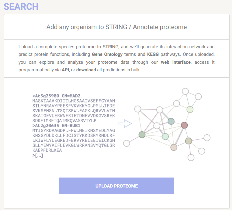
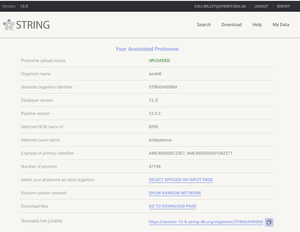
Using the STRING web tool, we will now peform ORA of this custom axolotl annotation. We will not perform GSEA on STRING purely in the interest of time, as the processing takes a lot longer than ORA, however if you wish to run this at a late date, please go ahead! The axolotl annotation link is persistent and citable, enhancing the reproducibility of your novel species FEA 🏆

Step 1: Open the following link in your browser:

https://version-12-0.string-db.org/organism/STRG0A90SNX

STRG0A90SNX is the annotation ID assigned by STRING.

This link will take you to the axolotl annotation page, where you can click SELECT SPECIES ON INPUT PAGE to add the custom species to the Organisms field, then toggle to your desired search type.

There is also a downloads page, where any of the STRING annotation files can be downloaded. If you wanted to use the STRING annotation files in clusterProfiler or WebGestaltR, you would download the ‘protein enrichment terms’ file and then extract the terms and axolotl gene IDs into the required formats, as we did for the emapper annotations.

STRING protein enrichment terms file format:

Step 2: On STRING, click SELECT SPECIES ON INPUT PAGE, then from the left search options, select Multiple proteins.

Note that the Organism field is pre-filled with STRG0A90SNX (axolotl).

Step 3: In the RStudio Files pane, locate your saved ORA gene list from earlier - workshop/Axolotl_DEGs.txt. Click the file to view it in RStudio, then copy paste the list into the STRING List of Names search field, then select SEARCH

Step 4: Click CONTINUE at the gene ID review page

Before we explore the results, note that we have performed ORA without a background gene list! 😮

There is no option at the query page (even under Advanced Settings) to provide a custom background gene list initially. This must be done after the initial search has been run. Hopefully this will change in future versions 🫠

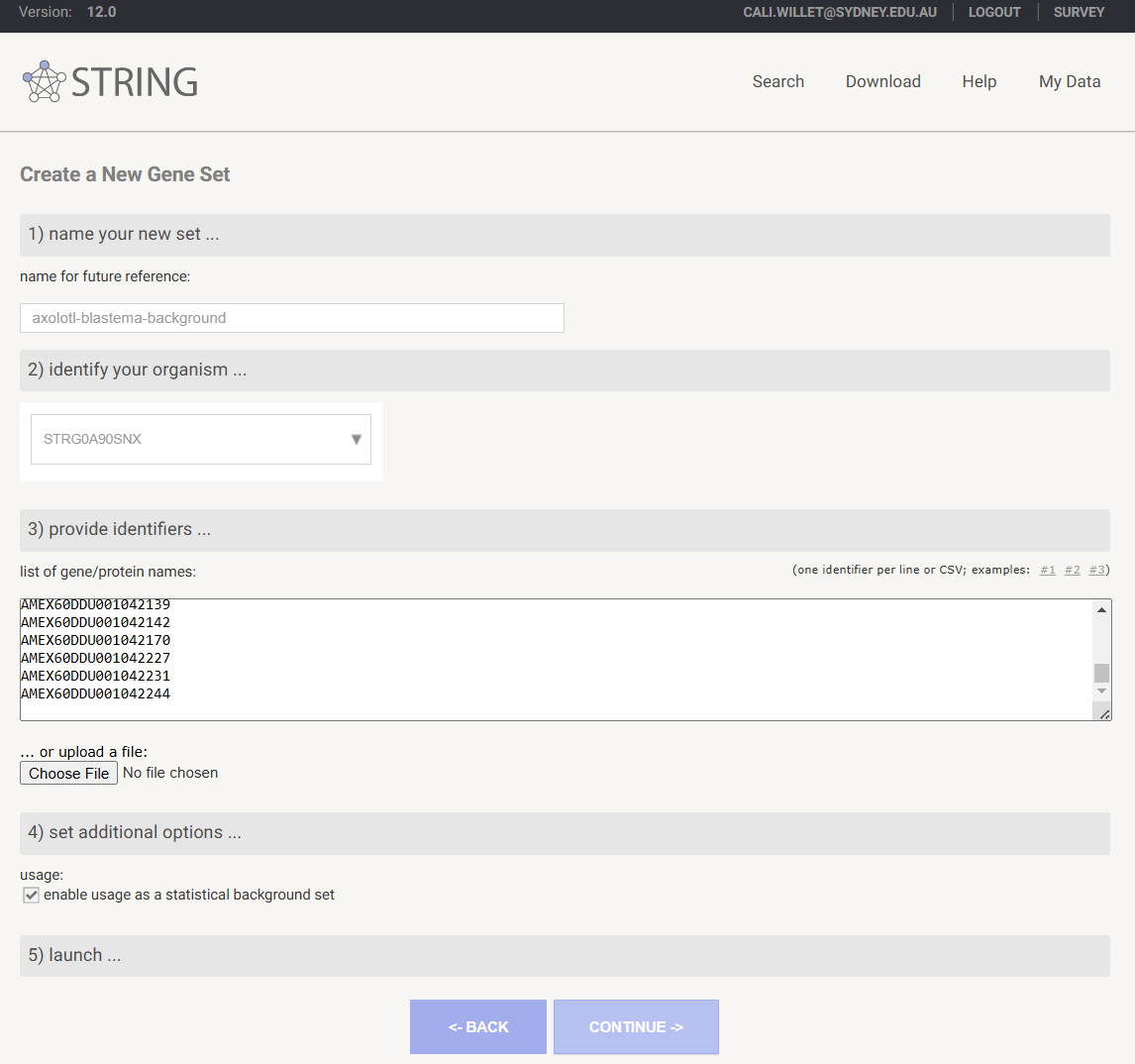
❗ In order to add or apply a previously saved custom background gene list, you need to be logged in to STRING. The upload can take a bit of time, so you do not need to do this now, however the dropdowns below provide instructions for applying a saved background or adding a new one.

Add a saved custom background to STRING analysis

After running ORA or GSEA, on the results page, click on the ANALYSIS tab
Scroll ALL the way to the bottom of the page to the subheading Statistical background
- If you do not have a relevant saved background gene list in your STRING saved datasets, you would select Add background. See next dropdown for details
- If you do have a relevant background saved, change Whole Genome to the relevant gene background list from the drop-down menu
Once you have selected the background, click UPDATE and the FEA will be re-computed using the custom statistical background

Save a new custom background gene list to your STRING profile

Under ANALYSIS tab of results page, at Statistical background, select ADD BACKGROUND
You will be prompted to login if you are not already
Under 1) name your new set provide a descriptive name for your background gene list
Select your organism at 2) identify your organism
At 3) provide identifiers copy your list of background IDs into the list of gene/protein names field
Ensure that enable usage as a statistical background is checked at 4) set additional options...
Click CONTINUE to map your IDs. This may take several minutes.

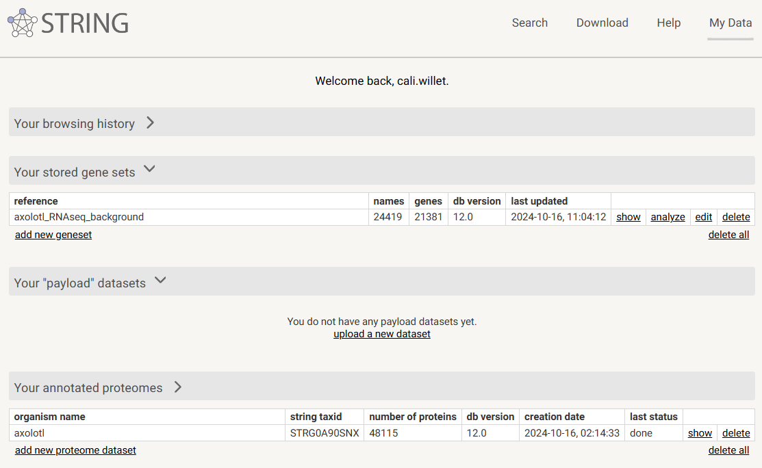
STRING saves your custom datasets under My Data:

Now let’s explore the results!

Some suggestions:

Select a node on the network, and then Show this node's terms in the analysis table to highlight the terms the gene was present in
Select the coloured lines connecting nodes to show evidence suggesting a functional link (all putative of course!)
Clicking on the Analysis tab will show the enrichment tables with results for GO, STRING, KEGG, Reactome, TISSUES and UniProt
Below the tables, under Functional enrichment visualization you can change Category to alter which database results are plotted

17.13.1 How do the STRING results compare to those we generated in R?

We expect a large difference in the results because of the differing proteome annotation methods - both the annotation tool and the databases that were annotated against.

The eggNOG emapper annotations we used in R rely on orthology-based predictions, employing extensive similarity searches to map genes to their closest evolutionary counterparts across diverse species. This results in a more comprehensive catalog of functional terms, even if they are inferred rather than directly evidenced.

In contrast, STRING’s custom species annotations are based on high-confidence protein-protein interaction networks and empirical data, which can narrow down the set of enriched pathways. We expect species bias to have a considerable effect when attempting to use this platform for novel species.

First of all we see a difference in the number of genes annotated to terms:

Method	GO	KEGG Pathways	All
emapper	21,373	12,226	39,536
STRING	36,895	21,502	38,398

And a clear lack of overlap in number of enriched GO terms and term IDs between STRING and the R tools:

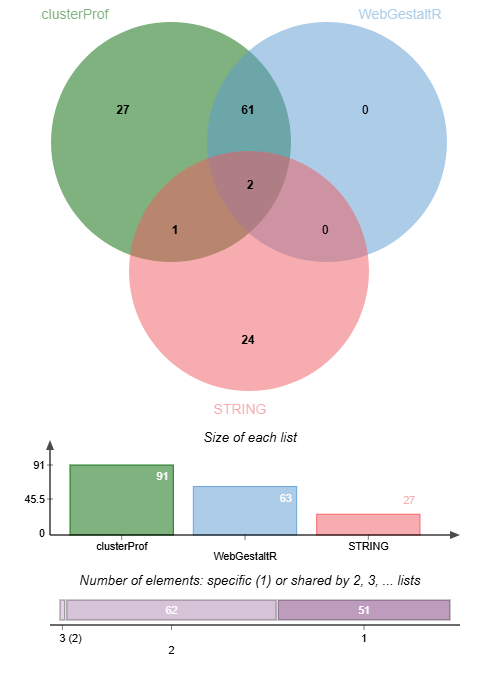
These GO terms from STRING may be parent terms of more specific child terms prevalent in the R output. For a real world analysis, it would be optimal to compare, and deduce whether both methods could provide valuable and complimentary insights, or whether the results from one annotation approach or the other were more suited to your novel species.

Whichever you choose, strength to you! This is not an easy space to work in 💪

Remember the importance of validating your results through other means! 🧪

17.14 End of activity summary

We have imported a custom emapper annotation, GO ontology, and KEGG Pathways file for a novel species (axolotl) not supported by any FEA tool
We have run clusterProfiler ORA of GO terms and GSEA of KEGG pathways using custom TERM2GENE/TERM2NAME files, and visualised results with enrichplot
We have run WebGestaltR ORA of GO terms and GSEA of KEGG pathways using custom .gmt/.des files, and explored the results in the interactive HTML report
We have run ORA on STRING web using a custom, persistent, citable proteome annotation
We have compared STRING and R-based results, and discussed why differing annotation methods and databases lead to divergent enrichment outcomes for novel species

16 clusterProfiler and enrichplot

18 Uncertainties of a functional enrichment analysis