7 Niche annotation using KNN

Load the psuedobulked cell type references

# A function to get the niche counts out of the Seurat objects
grab_nichecounts <- function(xenium_object, k_param, cell_types, fov ="fov"){
  
  # Steal from the Seurat BuildNicheAssay function to get nearest neighbours
  
  coords <- GetTissueCoordinates(xenium_object[[fov]], which = "centroids")
  cells <- coords$cell
  rownames(coords) <- cells
  coords <- as.matrix(coords[, c("x", "y")])
  neighbors <- FindNeighbors(coords, k.param = k_param)
  ct.mtx <- matrix(data = 0, nrow = length(cells), ncol = length(unlist(unique(xenium_object[[cell_types]]))))
  rownames(ct.mtx) <- cells
  colnames(ct.mtx) <- unique(unlist(xenium_object[[cell_types]]))
  cts <- xenium_object[[cell_types]]
  for (i in 1:length(cells)) {
    ct <- as.character(cts[cells[[i]], ])
    ct.mtx[cells[[i]], ct] <- 1
  }
  niche_counts <- as.matrix(neighbors$nn %*% ct.mtx)%>%t()
  niche_counts[1:5,1:5]
  
  return(niche_counts)
  
}

Get each cell’s 50 neareast neighbours

p1_nichecounts_detailed <- grab_nichecounts(cropped.obj, 50,cell_types = "MMR_atlas_lowlevel_pred", fov = "zoom")
p1_nichecounts_detailed[1:5,1:5]
#>                            bggahoon-1 bggaimpb-1 bggalkpc-1
#> cE01 (Stem/TA-like)                17         18         17
#> cE03 (Stem/TA-like prolif)         30         31         29
#> cE11 (Enteroendocrine)              0          0          0
#> cM06 (DC IL22RA2)                   0          0          0
#> cTNI24 (NK GZMK+)                   0          0          0
#>                            bggbeool-1 bggbnono-1
#> cE01 (Stem/TA-like)                18         16
#> cE03 (Stem/TA-like prolif)         30         28
#> cE11 (Enteroendocrine)              0          0
#> cM06 (DC IL22RA2)                   0          0
#> cTNI24 (NK GZMK+)                   0          0

Variable features (cell types) in the data

combined_niche_seu <- CreateSeuratObject(p1_nichecounts_detailed)
combined_niche_seu <- NormalizeData(combined_niche_seu, scale.factor =1)

combined_niche_seu <- FindVariableFeatures(combined_niche_seu)

top20 <- head(VariableFeatures(combined_niche_seu), 20)

plot1 <- VariableFeaturePlot(combined_niche_seu)
plot2 <- LabelPoints(plot = plot1, points = top20, repel = TRUE)

plot2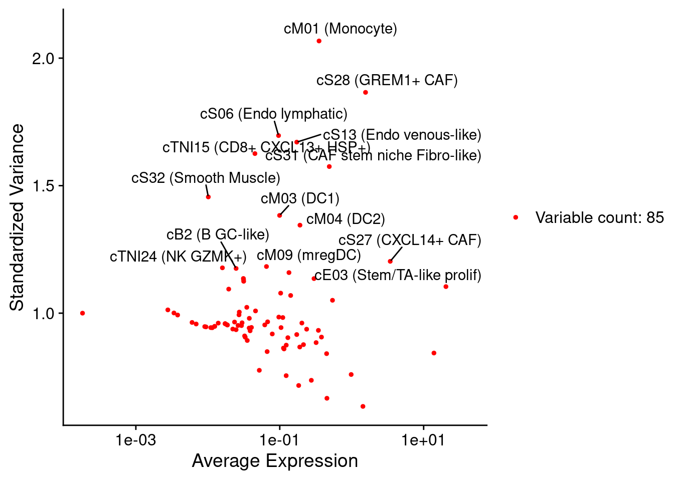

Elbow plot of niche-level PCA

combined_niche_seu <- ScaleData(combined_niche_seu)
combined_niche_seu <- RunPCA(combined_niche_seu, features = VariableFeatures(object = combined_niche_seu))
DimPlot(combined_niche_seu, reduction = "pca") + NoLegend()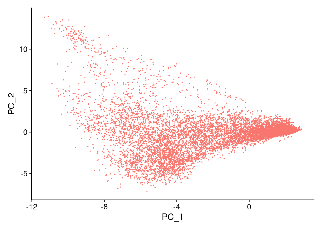

ElbowPlot(combined_niche_seu,ndims = 30)+
   geom_vline(xintercept = 5, colour="blue", linetype = "longdash")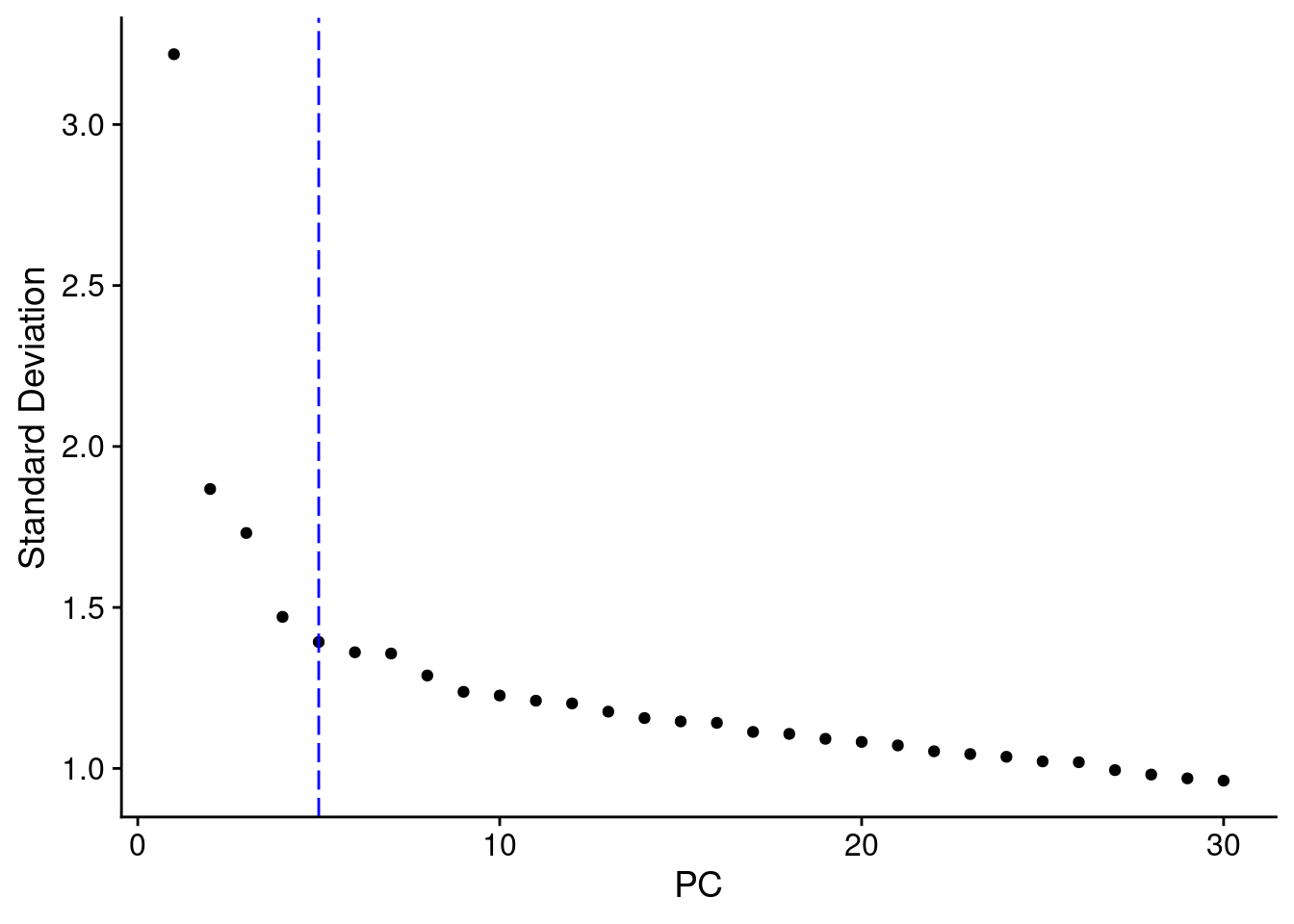

UMAP of KNN matrix

# Even running this with 10 PCs look ok, but maybe a bit complicated
combined_niche_seu <- FindNeighbors(combined_niche_seu, dims = 1:5)
# Setting a low resolution so we don't end up with an unmanageable number of niches
combined_niche_seu <- FindClusters(combined_niche_seu)
#> Modularity Optimizer version 1.3.0 by Ludo Waltman and Nees Jan van Eck
#> 
#> Number of nodes: 16537
#> Number of edges: 449088
#> 
#> Running Louvain algorithm...
#> Maximum modularity in 10 random starts: 0.9618
#> Number of communities: 64
#> Elapsed time: 1 seconds
combined_niche_seu <- FindClusters(combined_niche_seu, resolution = 0.1)
#> Modularity Optimizer version 1.3.0 by Ludo Waltman and Nees Jan van Eck
#> 
#> Number of nodes: 16537
#> Number of edges: 449088
#> 
#> Running Louvain algorithm...
#> Maximum modularity in 10 random starts: 0.9869
#> Number of communities: 36
#> Elapsed time: 1 seconds
combined_niche_seu <- RunUMAP(combined_niche_seu, dims = 1:5)

DimPlot(combined_niche_seu, reduction = "umap", group.by = "seurat_clusters", label = T)+NoLegend()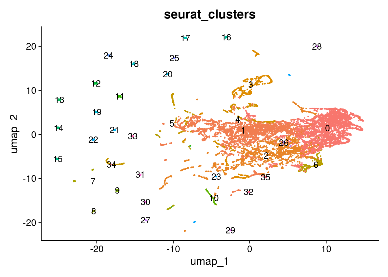

marks <- FindAllMarkers(combined_niche_seu)

Plot the niches on the slide

# Check everything lines up
all.equal(colnames(combined_niche_seu), colnames(cropped.obj))
#> [1] TRUE

cropped.obj$Niche <- combined_niche_seu$seurat_clusters

# Plot the 42 predicted niches
plot <- ImageDimPlot(cropped.obj,fov = "zoom", group.by = "Niche", 
                     size = 0.3, cols = "polychrome",
                     dark.background = T, boundaries = "segmentation",border.size = 0.1,
                     nmols = 20000) + 
  ggtitle("Niches")

plot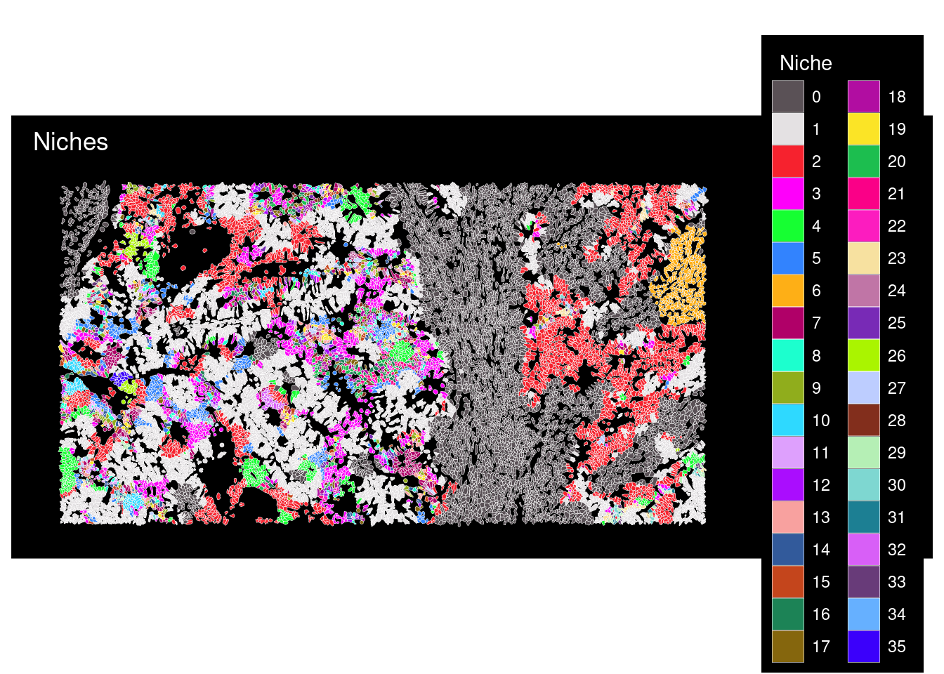

7.1 Plot the niche composition in terms of cell type makeup

niche_makeup_gut <- cropped.obj@meta.data %>%
  group_by(Niche) %>%
  mutate(Total = n()) %>%
  group_by(MMR_atlas_midlevel_pred, Niche, Total) %>%
  summarise(Count = n(), .groups = "drop") %>%
  mutate(Niche_pct = Count / Total * 100) %>%
  arrange(Niche) %>%
  mutate(Niche = factor(Niche, levels = unique(Niche)))

# Auto name the niches
niche_names <- niche_makeup_gut %>%
  group_by(Niche) %>%
  arrange(desc(Niche_pct), .by_group = TRUE) %>%
  slice_head(n = 3) %>%
  mutate(label = paste0(MMR_atlas_midlevel_pred, " (", round(Niche_pct), "%)")) %>%
  summarise(Niche_name = paste(label, collapse = " – "), .groups = "drop")

niche_makeup_gut <- niche_makeup_gut %>%
  left_join(niche_names, by = "Niche")

# Create a mapping vector from cluster to name
niche_name_vec <- setNames(niche_names$Niche_name, niche_names$Niche)

# Assign to metadata
cropped.obj$Niche_named <-as.character(niche_name_vec[as.character(cropped.obj$Niche)])

ggplot(data = niche_makeup_gut, aes(x = Niche, y = Niche_pct, fill = MMR_atlas_midlevel_pred))+
  geom_bar(stat = "identity")+
  labs(x = "Niche", y = "Celltype % of niche", fill = "Cell type")+
  blank_theme+
  theme(axis.text.x = element_text(angle = 90, vjust = 0.5, hjust=1))