4 Preprocessing Xenium
Load required libraries
library(tidyverse)
library(Seurat)
library(future)
library(qs)
library(SingleR)
library(harmony)
library(scider)
library(SpatialExperiment)
library(FNN)
library(limma)
library(edgeR)
library(Glimma)
library(parallel)
library(GSA)
Set basic ggplot2 themes for all plots and cell type colours.
blank_theme <- theme_bw(base_size = 7)+
  theme(panel.grid=element_blank(),
        strip.background = element_blank(),
        plot.title = element_text(size=7))

plan("multisession", workers = 10)
options(future.globals.maxSize = 12000 * 1024^2)

cell_types <- c("Epi", "Plasma", "Fibro", "Peri", "Macro", "Granulo", "TCD4", "SmoothMuscle", "Endo",
                "B", "DC", "ILC", "Schwann", "Mast", "Mono", "TCD8", "NK", "TZBTB16", "Tgd","QC_fail")

colors <- c("#DEA0FD", "green", "#f99379", "yellowgreen","#654522" ,"#dcd300", "#fdbf6f", "#b2df8a" ,"#CC79A7","#cab2d6",
            "#6a3d9a", "#1f78b4", "#85660D", "#2b3d26","#D55E00", "#a6cee3","darkblue","lightpink", "#1C7F93",
            "grey")

cell_type_colors <- setNames(colors, cell_types)
4.1 Xenium data
To get more information about the data generated by Xenium instrument visit: Understanding Xenium outputs
With the folder we are working we have the following structure:
data/Xenium/Sample_P1/
├── analysis_summary.html
├── analysis.zarr.zip
├── cell_boundaries.csv.gz
├── cell_boundaries.parquet
├── cell_feature_matrix.h5
├── cell_feature_matrix.zarr.zip
├── cells.csv.gz
├── cells.parquet
├── cells.zarr.zip
├── experiment.xenium
├── gene_panel.json
├── metrics_summary.csv
├── morphology_focus
│   ├── morphology_focus_0000.ome.tif
│   ├── morphology_focus_0001.ome.tif
│   ├── morphology_focus_0002.ome.tif
│   └── morphology_focus_0003.ome.tif
└── nucleus_boundaries.csv.gz
analysis_summary.html: Static QC/analysis report generated by the pipeline (read depth, % reads mapped to panel, cell counts, clustering/dim‑red snapshots, etc.). Good for a quick health check of the run.
analysis.zarr.zip: A zipped Zarr store holding analysis artifacts (e.g., dimensionality reductions, clusters, embeddings, annotations). Use from Python with zarr/xarray; handy for chunked, lazy I/O.
cell_boundaries.csv.gz: Per‑cell polygon coordinates (often one row per vertex with a cell_id, x, y, maybe vertex_index). Use to draw cell outlines in viewers or to compute spatial features (areas, neighbor graphs).
cell_boundaries.parquet: Same information as above but in Apache Parquet (columnar, compressed, faster to load/filter). Prefer this for programmatic work.
cell_feature_matrix.h5: (HDF5) Sparse counts matrix of cells × features (genes/probes/segments). Load with h5py/scanpy in Python or rhdf5 in R. Canonical input to most downstream tools.
cell_feature_matrix.zarr.zip: Same matrix as above, but in Zarr. Better for cloud / chunked access and parallel reads.
cells.csv.gz: Per‑cell metadata table: cell IDs, positions (centroid x/y), QC metrics (UMIs, genes detected), segmentation areas, cluster labels, etc.
cells.parquet: Same as above, columnar & faster. Usually the one you want to script against.
cells.zarr.zip: Zarr version of the per‑cell metadata (again, for scalable / cloud workflows).
experiment.xenium: 10x’s binary container with raw & processed assay data plus run metadata. Used by 10x/partner software to (re)generate the other derivatives; you typically don’t parse this directly unless using 10x tooling.
gene_panel.json: The targeted probe set definition: gene symbols, number of probes per gene, probe sequences/IDs, sometimes categories (positive controls, negatives). Useful to map feature IDs back to genes.
metrics_summary.csv: Run‑level QC metrics aggregated across the experiment (number of transcripts, % on‑panel, cells detected, median counts per cell, etc.). Good for at‑a‑glance comparisons between experiments.
morphology_focus/: High‑resolution morphology images (often nuclear stain / DAPI or brightfield) in OME‑TIFF tiles:
- morphology_focus_0000.ome.tif
- morphology_focus_0001.ome.tif
- morphology_focus_0002.ome.tif
- morphology_focus_0003.ome.tif
Use to visualize tissue context, overlay cell/nucleus boundaries, or extract image features.
nucleus_boundaries.csv.gz: Polygon coordinates for nucleus segmentations (analogous to cell_boundaries.*). Useful if you want nucleus‑specific morphometrics or to distinguish nucleus vs whole‑cell masks.
Set output directory path
outdir <- "./xenium_results"
dir.create(file.path(outdir), showWarnings = FALSE)
Set slide path
path <- "./data/Xenium/Sample_P1/"Load the Xenium data
xenium.obj <- LoadXenium(path, fov = "fov")4.2 Quality Controls
Remove cells with 0 counts: We remove cells with zero transcript counts (nCount_Xenium == 0) as these typically represent empty or mis-segmented regions with no detectable expression. Including such cells can introduce noise, distort downstream analyses like clustering or normalization, and increase computational burden. Filtering them ensures that only biologically meaningful cells are retained for analysis.
xenium.obj <- subset(xenium.obj, subset = nCount_Xenium > 0)Plot the raw counts
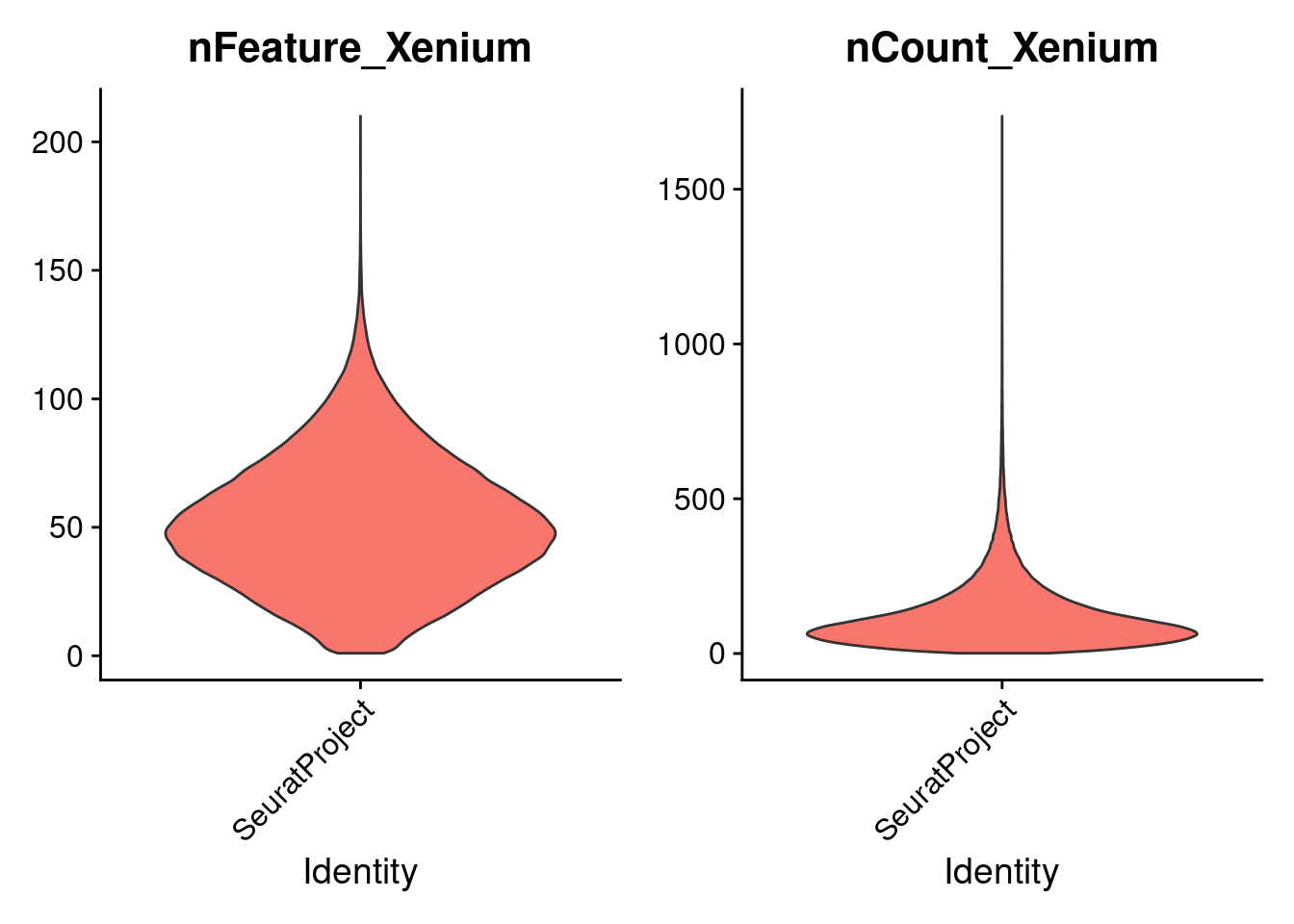
Look at some attributes of the Seurat object
xenium.obj@assays$Xenium$counts[1:5,1:5]
#> 5 x 5 sparse Matrix of class "dgCMatrix"
#>        aaaadaba-1 aaaadgga-1 aaaadmca-1 aaaaenln-1
#> ABCC8           .          .          .          .
#> ACP5            .          .          .          .
#> ACTA2           2          1          .          .
#> ADH1C           .          .          .          .
#> ADRA2A          .          .          .          .
#>        aaaajoff-1
#> ABCC8           .
#> ACP5            1
#> ACTA2           .
#> ADH1C           .
#> ADRA2A          .
head(rownames(xenium.obj))
#> [1] "ABCC8"   "ACP5"    "ACTA2"   "ADH1C"   "ADRA2A"
#> [6] "AFAP1L2"
Look at some key colorectal cancer (CRC) gene markers on the slide image
ImageDimPlot(xenium.obj, fov = "fov", molecules = c("PIGR", "LGR5", "GUCA2A", "GUCA2B", "OLFM4", "TGFBI"),axes = TRUE, nmols = 20000)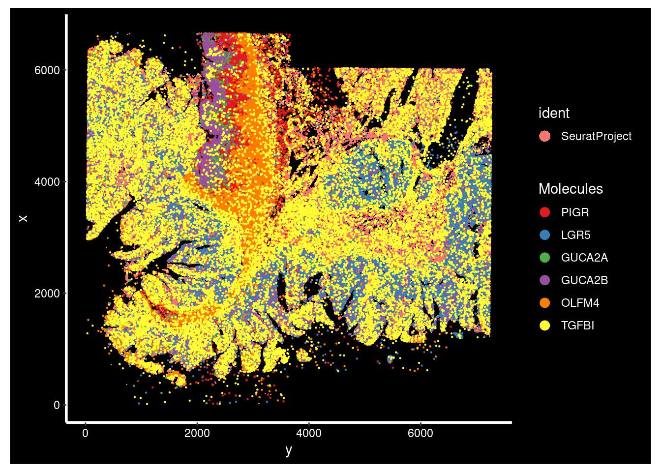
Get a small subset of the data, crop a part of the slide
cropped.coords <- Crop(xenium.obj[["fov"]], x = c(100,2000), y = c(5000, 6000), coords = "plot")
xenium.obj[["zoom"]] <- cropped.coords
Visualise cropped area with cell segmentations & selected molecules
DefaultBoundary(xenium.obj[["zoom"]]) <- "segmentation"
ImageDimPlot(xenium.obj, fov = "zoom", axes = TRUE, border.color = "white", border.size = 0.1,
coord.fixed = FALSE, molecules = c("PIGR", "LGR5", "GUCA2A", "GUCA2B", "OLFM4", "TGFBI"), nmols = 10000)
cropped.cells <- xenium.obj@images$zoom$centroids@cells
cropped.obj <- subset(xenium.obj, cells = cropped.cells)
# Make the object a lot smaller by dropping the full fov
cropped.obj[['fov']] <- NULL
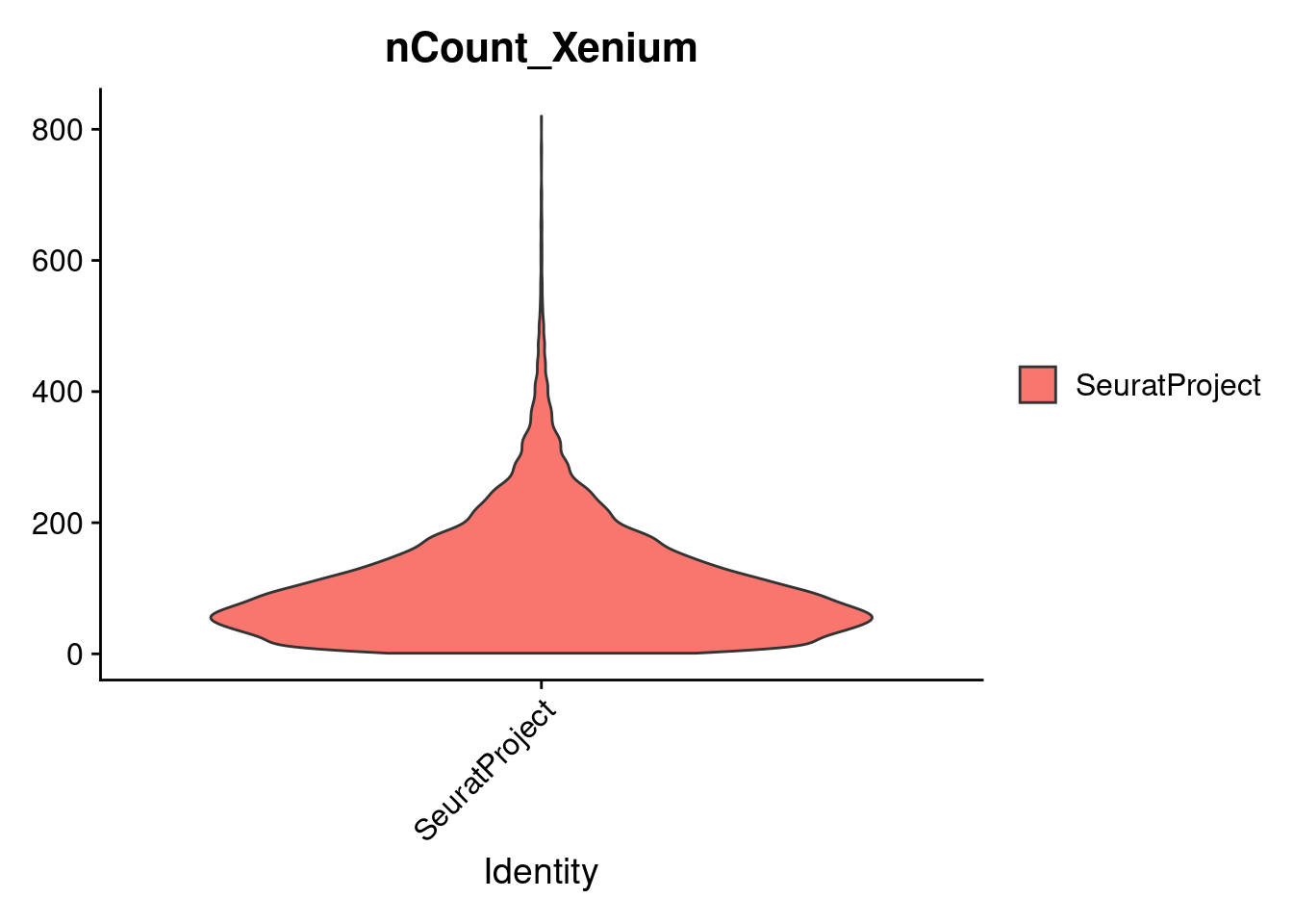
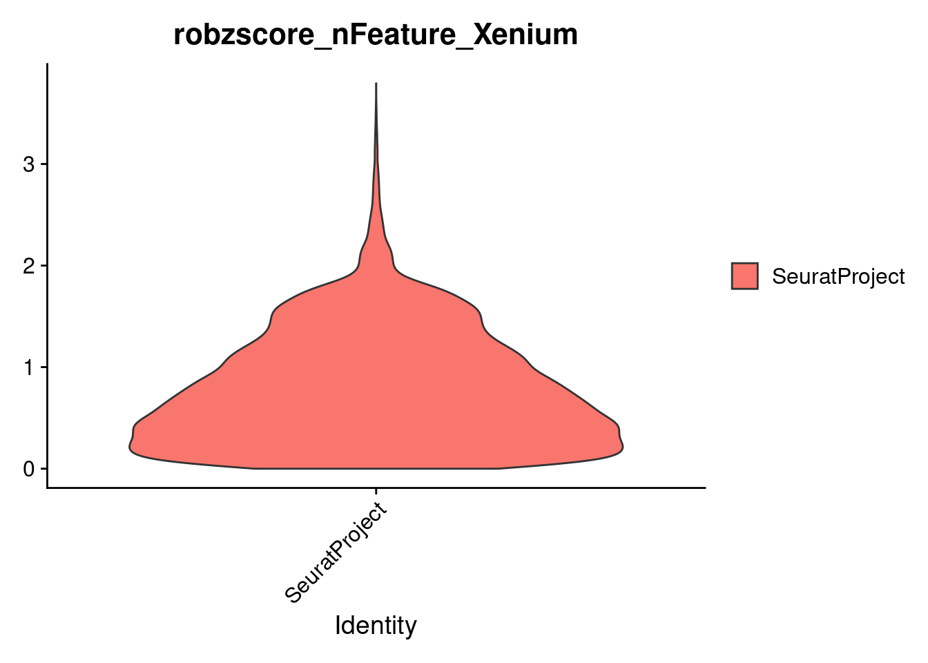
#qsave(cropped.obj, "./data/Xenium/preprocessed/Cropped_P1.qs")Calculate the median absolute deviation (MAD) values for counts features
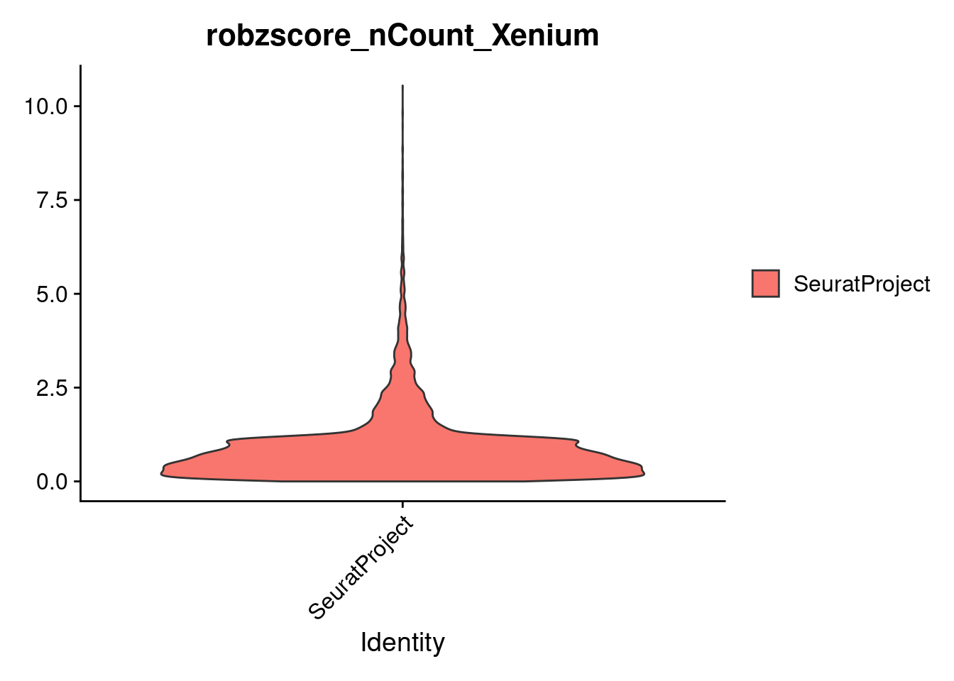
To identify and remove outlier cells, we compute the MAD for each of two quality control metrics:
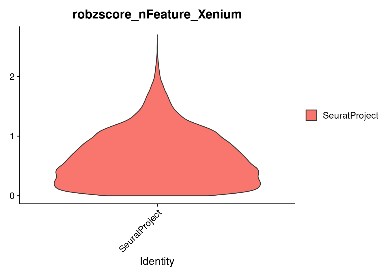
nFeature_Xenium (number of detected genes)
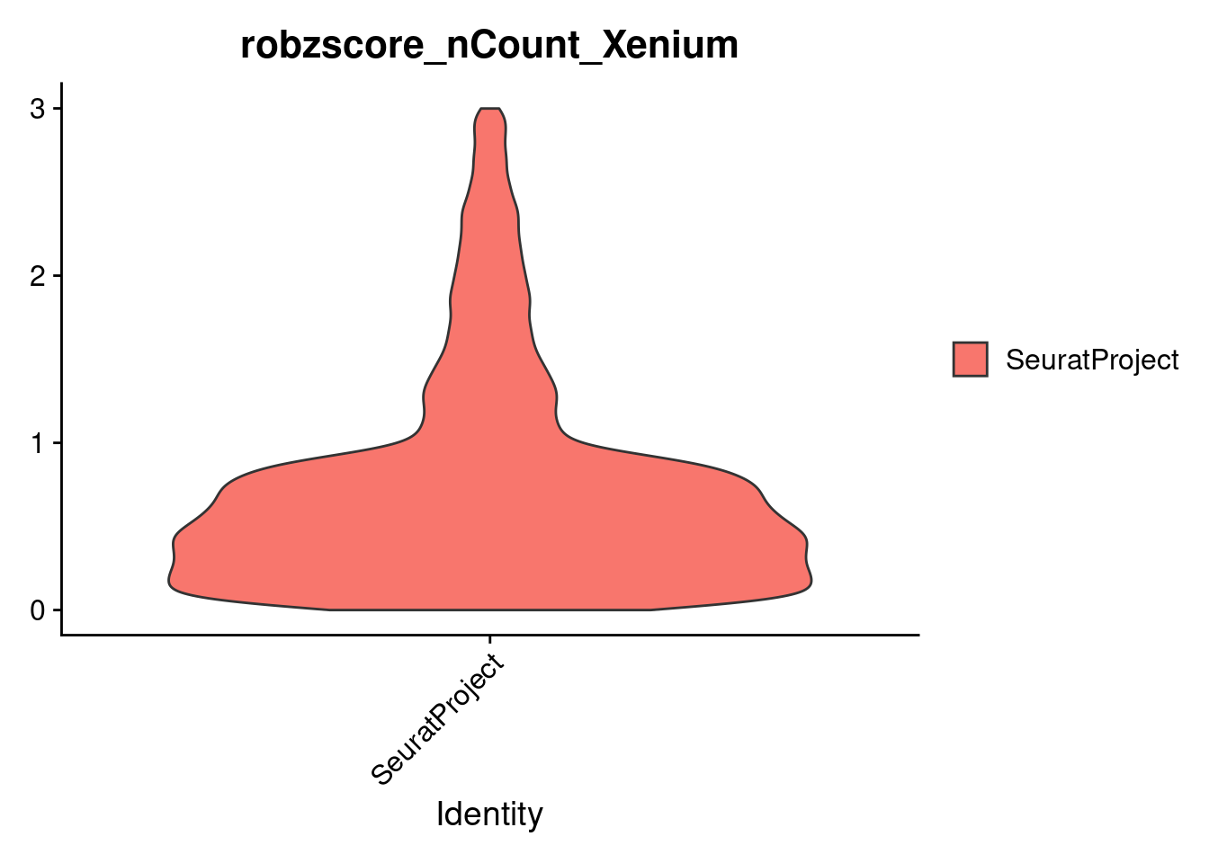
nCount_Xenium (total number of transcripts)
MAD is a robust measure of variability, less influenced by extreme values than standard deviation. We then calculate robust Z-scores to flag cells that deviate strongly from the median, allowing us to filter out low-quality or noisy cells.
cropped.obj <- qread("./data/Xenium/preprocessed/Cropped_P1.qs")

md <- cropped.obj@meta.data%>%
  rownames_to_column("Barcode")%>%
  mutate(m = median(nFeature_Xenium))%>%
  mutate(s = mad(nFeature_Xenium))%>%
  mutate(robzscore_nFeature_Xenium = abs((nFeature_Xenium - m) / (s)))%>%
  mutate(m = median(nCount_Xenium))%>%
  mutate(s = mad(nCount_Xenium))%>%
  mutate(robzscore_nCount_Xenium = abs((nCount_Xenium - m) / (s)))%>%
  ungroup()%>%
  data.frame()
Reset the rownames
rownames(md) <- md$Barcode
cropped.obj@meta.data <- md
Subset based on robust Z score cutoffs
dim(cropped.obj)
#> [1]   422 19437

cropped.obj <- subset(cropped.obj, subset = robzscore_nFeature_Xenium < min_QC_robz & robzscore_nCount_Xenium < min_QC_robz & nCount_Xenium > 20)

VlnPlot(cropped.obj, features = c("nCount_Xenium"), pt.size = -1)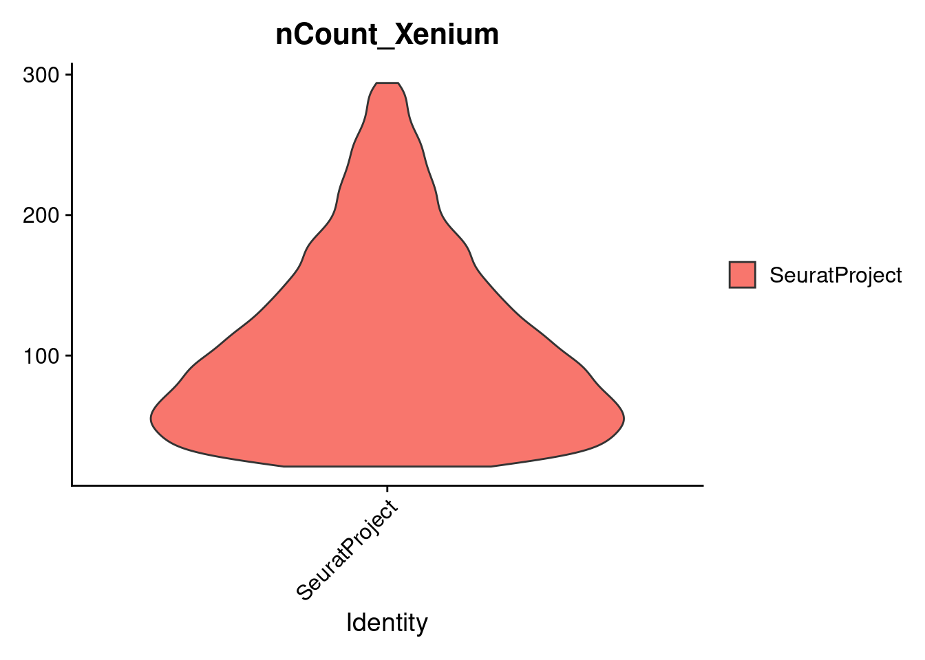
dim(cropped.obj)
#> [1]   422 16537