8 Online Tools
Functional enrichment analysis can be performed using various web-based tools, each of which is designed to meet specific analytical needs. These tools often vary in the databases they use, their statistical approaches, and their capabilities to perform different types of analysis, such as Over-Representation Analysis (ORA) or Gene Set Enrichment Analysis (GSEA).
In this workshop, we will explore several popular tools for functional enrichment analysis, including gProfiler, STRING, Reactome, and MSigDB GSEA. Each tool offers unique features and insights, providing flexibility in selecting the right method for diverse datasets and research questions.
8.1 FEA in gProfiler 
gProfiler is known for its integration of numerous species and databases. It supports both ORA and GSEA, enabling users to assess Gene Ontology (GO), biological pathways, regulatory motifs and protein databases. With gProfile one can
8.1.1 Steps to perform ORA in g:Profiler:
- Prepare Input List: Ensure your input is formatted as one gene per line or in a suitable format for g:Profiler.
- Input Gene List: Paste your prepared gene list directly into the input box on the g:Profiler web page or upload a file containing your list.
- Select Organism: Choose the appropriate organism from the Organism dropdown menu (e.g., Homo sapiens for human data).
- Choose Statistical Domain Scope: Under Advanced options, select your preferred statistical background from the Statistical domain scope menu.If you choose “Custom” background, provide your custom background list by pasting or uploading the relevant file.
- Set Significance Threshold: Select the desired significance threshold method, such as g:SCS, Bonferroni, or Benjamini-Hochberg. - Specify the threshold value (e.g., 0.05, 0.1, etc.).
- Select Functional Annotation Databases: Navigate to the Data sources tab and choose one or more databases for analysis. Available options include:
- Gene Ontology (GO): Biological Process, Molecular Function, and Cellular Component.
- KEGG Pathways
- Reactome Pathways
- WikiPathways
- TRANSFAC
- mirTarBase
- Human Protein Atlas
- CORUM
- Human Phenotype Ontology (HP)
- Run Query: Run the analysis and review the enriched terms, pathways, and visual outputs. Download the results as needed for further exploration.
8.1.1.1 Browse the gProfiler Results
Overview: The analysis provided a comprehensive list of enriched terms across selected databases, highlighting significant GO. The results give a high-level summary of pathways or terms most relevant to the input data.
Detailed Results: The detailed results section includes a tabulated format with enriched terms, adjusted p-values, and relevant statistics. Each entry provides information such as the enrichment score, associated genes, and functional annotations, allowing for an in-depth understanding of biological significance.
GO Context: The Gene Ontology (GO) context is divided into three main categories: Biological Process (BP), Molecular Function (MF), and Cellular Component (CC). The analysis identifies which GO terms are significantly enriched, offering insights into the broader biological implications of the gene set. This helps in pinpointing processes such as cellular responses, metabolic pathways, and molecular interactions.
Query Info: This section includes specifics about the input data, including the total number of queried genes and any identifiers not recognised or mapped. It also details the statistical background used, the chosen organism, and other analysis settings, ensuring transparency and reproducibility of the results.
8.1.2 Steps to perform GSEA in g:Profiler:
- Prepare Your Pre-ranked List: Steps to provide a ranked gene list are given here.
- Input Gene List: Paste your prepared gene list directly into the input box on the g:Profiler web page or upload a file containing your list.
- Select Organism: Same as above.
- Select Ordered query: The “Ordered query” option in g:Profiler is designed to work with pre-ranked gene lists.
- Set Significance Threshold: Same as above.
- Provide a Custom GMT: This GMT file can be downloaded from MSigDB.
- Run Query: Same as above.
Challenge: GSEA with gProfiler
Download the Hallmark gene sets (h.all.v2024.1.Hs.symbols.gmt) from MSigDB and use it as Custom GMT.
8.2 FEA in STRING 
STRING (Search Tool for the Retrieval of Interacting Genes/Proteins) is a resource for exploring protein-protein interaction (PPI) networks. It combines experimental data, predictions, and curated information to build networks that highlight functional relationships, helping to reveal shared pathways or biological processes within gene or protein lists.
8.2.1 Steps to Perform ORA in STRING:
- Select Multiple proteins tab.
- Input Gene List: Paste your prepared gene list directly into the input box on the STRING web page or upload a file containing your list.
- Select Organism: Choose the appropriate organism from the Organisms dropdown menu (e.g., Homo sapiens for human data). STRING would auto-detect the organism if ENSEMBL IDs provided.
- Modify Settings: Under Advanced Settings, you can modify Required score from low (0.15) to highest (0.9) confidence. Similarly FDR stringency and Network type can be selected.
NOTE: In cases where long list of features is provided, STRING may chnage some of its settings so that:
- the nodes will have a simplified (not 3D) design
- previews of protein structures are not shown
- the network edges show interaction confidence only
8.2.2 Browse the STRING ORA Results
STRING generates multiple tabs as output, shown here:

Figure 8.1: Results tabs in STRING
8.2.2.1 Viewers
Under the Viewers tab, various visualisation layouts are available, with the Network option being the most notable and widely used.
8.2.2.2 Legend
The Legend tab offers a guide to the colors of nodes and edges, along with annotations for each individual query in the input list.

Figure 8.2: Nodes and edges colour-coded
8.2.2.3 Settings
In the Settings tab of the STRING results, users have the flexibility to adjust existing settings and apply new filters to customise their data view and analysis. This tab you to switch between network types, strengths, data sources, intertaction scores and more.
8.2.2.4 Analysis
One of the most essential tabs is the Analysis tab, which offers comprehensive functional enrichment analysis from a range of databases. These include Gene Ontology (GO) for biological processes, molecular functions, and cellular components; Pathway enrichment from sources such as KEGG, Reactome, and WikiPathways; and other significant data sources such as Human Phenotype annotations and UniProt for protein function and structure.
Columns of the STRING enrichment table are explained as following:
- Count In Network: The first number indicates how many proteins in your network are annotated with a particular term. The second number indicates how many proteins in total (in your network and in the background) have this term assigned. You can click on the numbers to see the network view of the gene sets behind them.
- Strength: Log10(observed / expected). This measure describes how large the enrichment effect is. It’s the ratio between i) the number of proteins in your network that are annotated with a term and ii) the number of proteins that we expect to be annotated with this term in a random network of the same size.
- Signal: The signal is defined as a weighted harmonic mean between the observed/expected ratio and -log(FDR). FDR tends to emphasise larger terms due to their potential for achieving lower p-values, while the observed/expected ratio highlights smaller terms, which have a high foreground to background ratio but cannot achieve low FDR values due to their size. The signal measure seeks to balance both metrics for a more intuittive ordering of enriched terms.
- False Discovery Rate: This measure describes how significant the enrichment is. Shown are p-values corrected for multiple testing within each category using the Benjamini–Hochberg procedure.
STRING visualises terms within each category using a bubble plot, effectively showcasing the significance and size of enriched terms. Additionally, it renders groups of related terms based on a user-defined similarity level, allowing users to identify clusters of functionally related terms within the data. This helps in interpreting complex enrichment results and highlighting key biological processes or pathways that are closely associated.
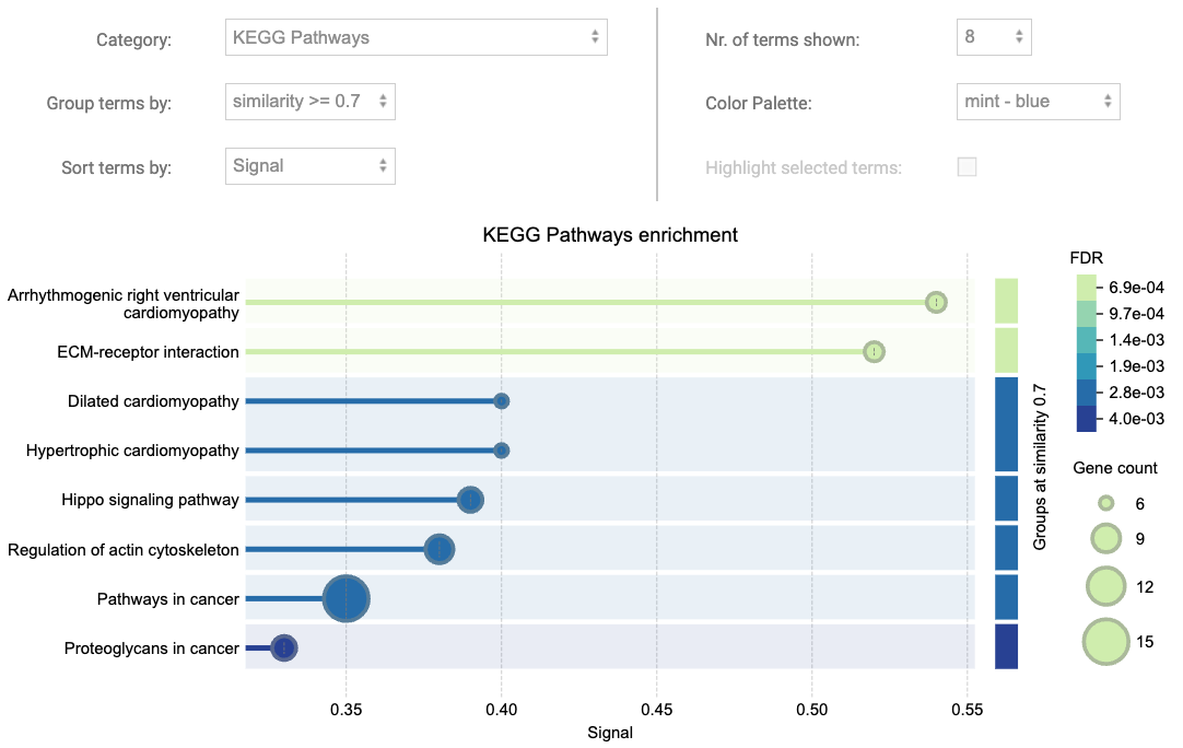
Figure 8.3: Functional enrichment visualisation with STRING
Analysis page, one can change the background including adding one of their own.

Figure 8.4: Statistical background
Finally the enriched terms can be downloaded at the end of the Analysis page, either individually per category or all enriched terms together.
8.2.2.5 Exports
The network data can be exported with the Exports tab. Also Network data can be directly sent to Cytoscape  for further networking. It is expected to have Cytoscape installed before exporting to it.
8.2.2.6 Clusters
The Clusters tab essentially provides three different types of clustering algorithms:
k-means clustering: Initialise k centroids randomly, assigns each data point to the nearest centroid, recompute the centroids as the mean of all points in a cluster until until centroids do not change significantly.
MCL clustering (Markov clustering): is a graph-based algorithm that uses flow simulation to detect clusters in a network by modeling random walks.
DBSCAN clustering: is a density-based algorithm that groups points closely packed together while marking points in low-density regions as outliers or noise
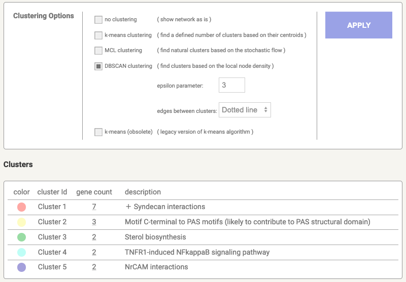
Figure 8.5: Network clustering in STRING
Clusters can be downloaded in .tsv format.
8.2.3 Steps to Perform GSEA in STRING:
- Selcet Proteins with Values/Ranks.
- Input Gene List: Paste your gene list with a meaningful value for ranking (fold-change, log-pvalue, abundance, …) directly into the input box on the STRING web page or upload a file containing your list of features and their corresponding values.
- Select Organism: Same as above.
- Advanced Setting: FDR stringency and the initial sort order can be set up in advance and hit the Search.
8.2.4 Browse the STRING GSEA Results
The output differs from ORA. For each gene set, the results include the enrichment score, its direction within the ranked list, the number of overlapping features with the gene set, and the associated FDR.
When a user selects a gene set from the enriched table,

Figure 8.6: An example table of WikiPathway gene sets
the associated genes are displayed within the ranking list. A table showing these genes along with their original ranking values is also provided.
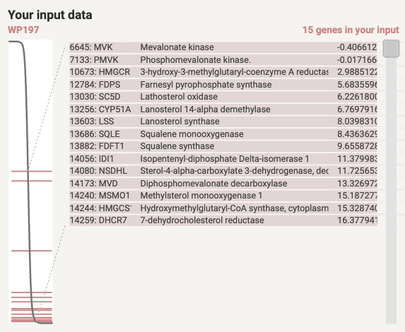
Figure 8.7: List of genes in the term (WP197) and their positions on the ranked list
Additionally, the locations of the corresponding proteins are highlighted in the proteome network:
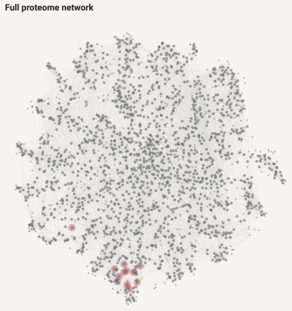
Figure 8.8: Proteome network
A Functional enrichment visualisation (similar to that of ORA) is provided at below the enriched tables.
Modify Enrichment display settings tab before downloading the enriched tables. It is recommended to merge terms with a certain level of similarity to reduce redundancy, especially if there are many overlapping terms.
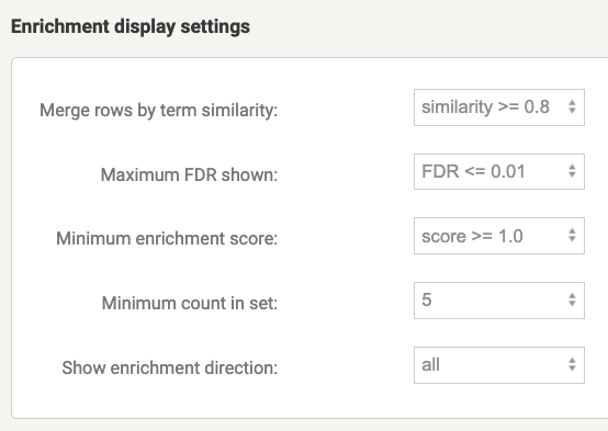
Figure 8.9: Enrichment display settings
Here is an example output of GSEA on STRING from a previous run (the link will expire in future).
8.3 FEA in GenePattern 
GenePattern, an online platform developed by the Broad Institute, offers a suite of tools for analyzing and visualizing genomic data, making bioinformatics accessible to researchers through a user-friendly, no-programming interface. Among its supported tools is Gene Set Enrichment Analysis (GSEA), which implements MSigDB GSEA analysis for identifying enriched gene sets in genomic data.
MSigDB (Molecular Signatures Database) is a collection of gene sets for Gene Set Enrichment Analysis, representing pathways and gene signatures linked to biological states or diseases. It helps identify enriched gene sets, aiding the analysis of gene expression changes and key pathways in experimental data.
8.3.1 Steps to Locate GSEA Module in GenePattern:
- Click on the Run button and then the Public Server

Figure 8.10: Navigate to Public Server
Sign in to GenePattern or Enter as Guest
Under
Modulestab hitBrowse ModulesFind gsea in the Browse Modules by Category page and hit GSEA
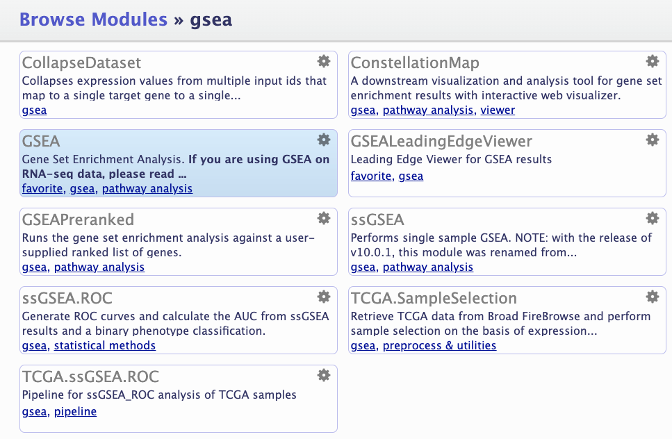
Figure 8.11: Browse GSEA module in GenePattern
8.3.2 Steps to Perform GSEA:
- Basic Parameters
- Create both .gct and .cls files following this scrit in R
- Load the .gct input file in the expression dataset tab and .cls file in the phenotype labels tab
- Select a .gmt file (Gene Matrix Transposed) from the gene sets database tab
- Set permutation under number of permutations tab
- Type of the permuattaion to be set under permutation type tab
- Select an appropriate DNA Chip annotation file from chip platform file tab
- Name the output file in output file name tab
- Advanced Parameters
- Scoring Scheme:
K-S: The score increment is the same for all genes in S regardless of their ranking or correlation strength.
WEighted: the score increment for each gene in S is weighted by its correlation with the phenotype, typically the absolute value of the correlation or ranking metric.
- Metric for ranking genes: Ranking metric of interest can be chosen from drop down menu. A detailed description od the metrics is given on GSEA-MSigDB Documentation.
Categorical Phenotypes: Signal-to-Noise Ratio, t-Test, Ratio of Classes, Log2 Ratio of Classes
Continuous Phenotypes: Pearson Correlation, Spearman Correlation
- Minimum and Maximum size of gene sets can be set using max gene set size and min gene set size tabs
8.3.2.1 Browse the GSEA results
Once the job has been queued and successfully run, the output will be listd on the left panel under Jobs tab:
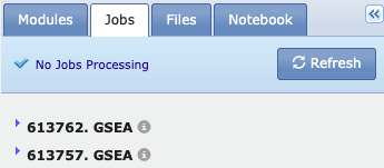
Figure 8.12: Job status in GenePattern
Of the most important files is the .zip file that was earlier specified under output file name tab in Basic parameters section which includes all the results. The results can also be navigated using the single files listed under the job id.
For Pezzini experiment, two html files generated for each of up- and down-regulated gene sets, something like:
gsea_report_for_Diff_1731388275794.html
gsea_report_for_Nodiff_1731388275794.html
The tabulated versions of the results are given in .tsv format:
gsea_report_for_Diff_1731388275794.tsv
gsea_report_for_Nodiff_1731388275794.tsv
The GSEA result tables have the following header and below is given details of one gene set:
| Parameter | Value |
|---|---|
| GS (follow link to MSigDB) | REACTOME_FRS_MEDIATED_FGFR2_SIGNALING |
| GS DETAILS | Details … |
| SIZE | 16 |
| ES | 0.83905387 |
| NES | 1.7128055 |
| NOM p-val | 0 |
| FDR q-val | 0.03902518 |
| FWER p-val | 0.648 |
| RANK AT MAX | 995 |
| LEADING EDGE | tags=38%, list=7%, signal=40% |
The leading edge column has three values:
- tags: 38% of the genes in the gene set are key to the enrichment result.
- list: These genes make up 7% of the total gene list being analyzed.
- signal: They contribute 40% of the enrichment signal, highlighting their importance in driving the association between this gene set and the biological phenotype being studied.
Challenge: How do different ranking metrics impact the output?
Run GSEA analysis using Hallmark gene sets with two metrics (tTest and Ratio_of_Classes). What are the upregulated terms (FDR < 0.1) in the Diff class, based on the t-test and Ratio of Classes metrics?
Question
Why might the HALLMARK_CHOLESTEROL_HOMEOSTASIS gene set be upregulated specifically in the differentiation condition of SH-SY5Y cells in Pezzini, et al 2016 experiment?
Show
- Relevance: Cholesterol is essential for neuronal function and membrane fluidity, particularly in processes like axonal growth and synapse formation. Neurons have a high demand for cholesterol, especially during differentiation when they extend axons and dendrites.
- Possible Insight: Upregulation of genes in this set could signify that differentiating cells are actively producing or transporting cholesterol to support membrane synthesis and cellular remodeling required for mature neuronal structures.
8.4 FEA in Reactome 
Reactome is an open-source database of curated biological pathways across species, offering pathway maps and enrichment tools to analyse gene lists in a pathway-focused context. It’s ideal for visualising data within established biochemical and cellular processes.
8.4.1 Steps to perform ORA in Reactome:
- Hit the
Analysis Toolstab

Figure 8.13: Analysis in Reactome
- Choose
Analyse gene listfrom the left panel
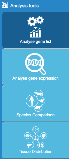
Figure 8.14: Analysis Tools in Reactome
Upload list of features on the box or choose a file, hit continue
-
Select prefered options:
- Project to Human: This option will convert identifiers from non-human species into human equivalents, allowing you to analyse data across species.
- Include interactors: This option integrates interactors from IntAct, a protein interaction database. Including interactors broadens the background network, potentially offering deeper insights.
Hit Analyse!
8.4.2 Steps to perform GSA in Reactome:
- If
Analyse gene expressionwas chosen instead, Reactome offers the following gene set analysis:

Figure 8.15: Ractome GSA
Lets try CAMERA as it represents the
camera()function oflimmapackage inRfor a gene set analysis.Choose TMM normalisation to ensure consistency with the input data used in other tools within our workshop.
Select data type and provide input data
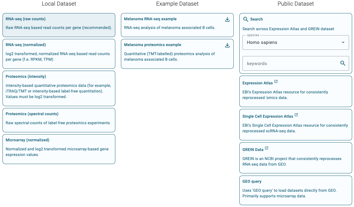
Figure 8.16: Ractome GSA - data type
- Annotate columns by adding extra info as follows:
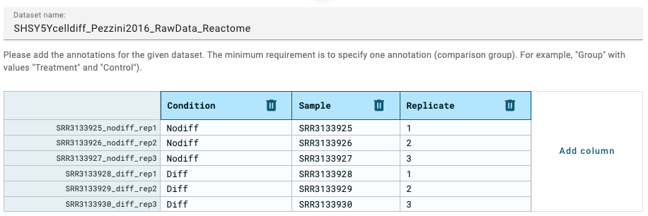
Figure 8.17: Pathway diagram
Save dataset and Continue
You can now browse the results
8.4.3 Browse the Reactome results
Results can be interactively browsed using the reactome pathway or voronoi visualisation modes: 
User can explore the pathway names listed in the table within the Analysis tab and they are displayed as popups on the pathway diagrams.
One can also select a pathway of interest by navigating through the left panel or by simply searching for the term in the search box.
The enriched table can be downloaded as shown below:

Figure 8.18: Table of ORA with Reactome
The diagram can be downloaded using this icons: 
Here is a sample pathway diagram from Reactome GSA.
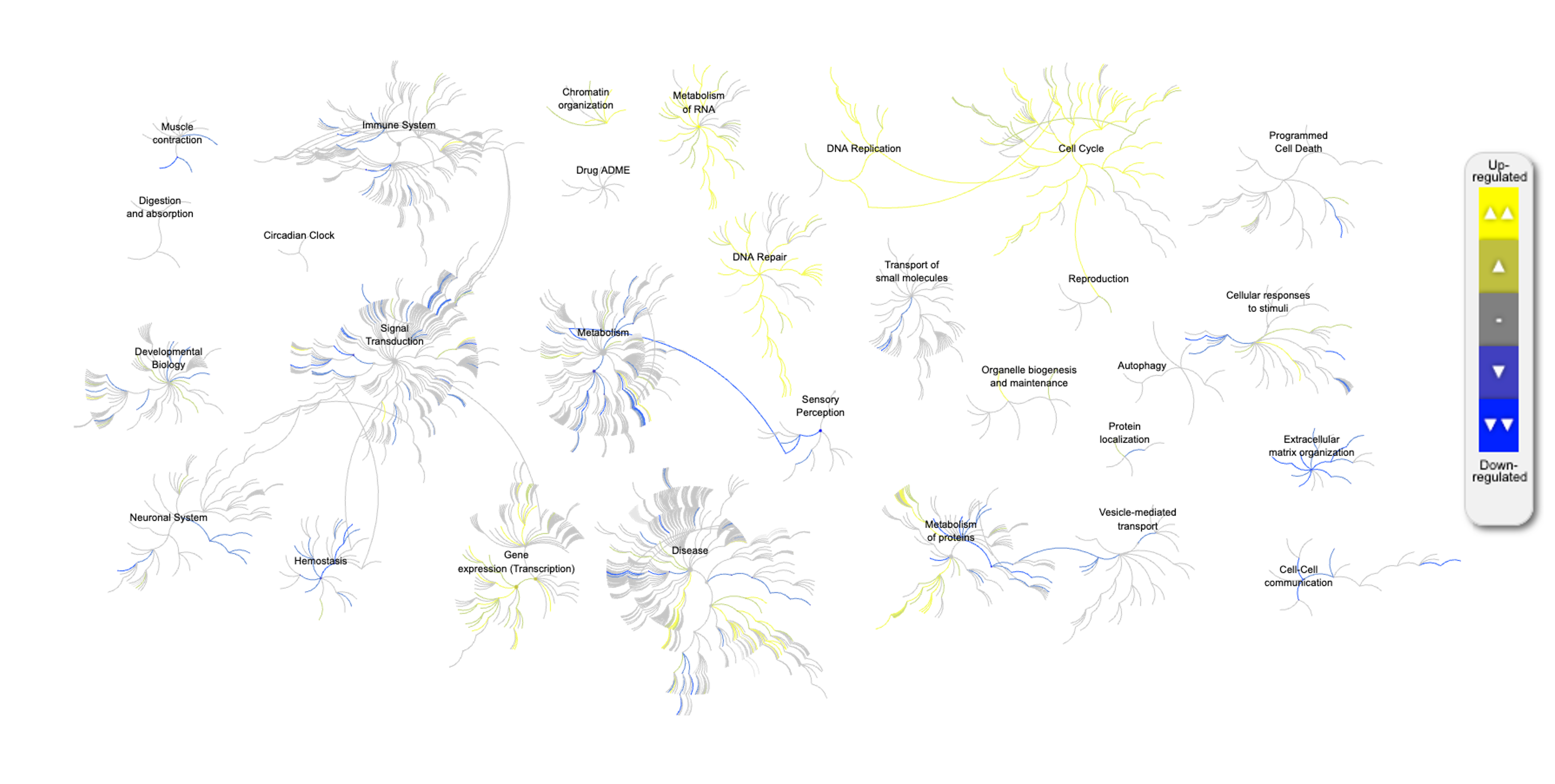
Figure 8.19: Pathway diagram - GSA
In case ssGSEA was selected, an overall output would look like below:
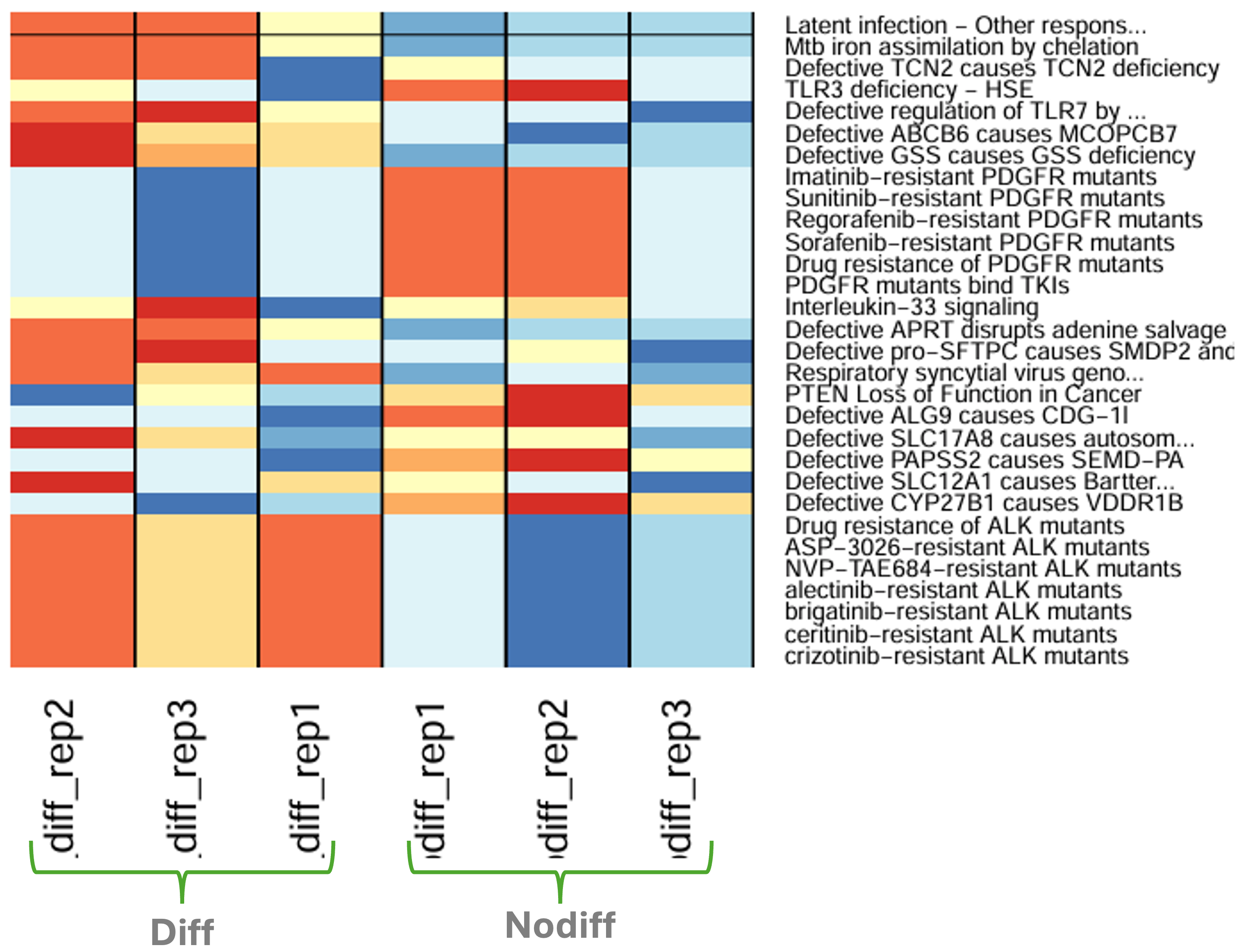
Figure 8.20: Expression of top 30 pathways with ssGSEA
8.5 Uncertainties of a functional enrichment analsysis
This section provides a summary of the paper by Wünsch et al. (2023), which explores uncertainties inherent in functional enrichment analysis. The study critically examines the sources of variability and challenges in this analytical approach, offering insights into improving its reliability and robustness.
Figure 8.21: From RNA sequencing measurements to the final results: A practical guide to navigating the choices and uncertainties of gene set analysis
8.5.1 Types of FEA
Functional enrichment analysis (FEA) typically involves one of over representation analysis (ORA), gene set enrichment analysis (GSEA) also known as functional class scoring (FCS), and Pathway Topology (PT).
- ORA
- ORA methods are the least complex among the three approaches of FEA.
- ORA methods requires a list of differentially expressed genes that are already analysed in differential expression analysis.
- The background population, the universe, can be a more general set of gene like those in human genome or more specific from thos observed in an experiment.
- A contingency table is created and the null distribution is modeled using the hypergeometric distribution.
- FCS
- FCS methods aim to aggregate the values of the gene-level statistics (ranks) into gene set-level statistic (enrichment score, ES).
- FCS can be classified as one of FCS I, those that take the expression data as input or FCS II that take a pre-ranked list of genes as input. With the latter, the information of the conditions (phenotypes) of the samples is lost, as such phenotype permutation cannot be performed leaving the choice of null hypothesis to gene set permutation.
- PT
- PT additionally models interactions between the genes. This approach generally scores considerably lower in terms of popularity in the reference database.
8.5.2 Considerations
- Pre-filter expression data: Exclude lowly expressed genes to improve statistical power.
- Handle gene IDs carefully: Convert gene IDs to the required format and remove any duplicates.
- Normalise expression data: Address sample-specific biases to enable fair comparisons between samples.
- Use appropriate methods for differential expression analysis: Recommended methods include limma (voom), DESeq2, and edgeR.
- Select suitable gene-level statistics: For FCS II, choose metrics like moderated t-statistic to rank genes meaningfully.
- Adjust for multiple testing: Ensure your analysis includes a correction for multiple hypothesis testing. Some methods require manual adjustments.
- Choose gene set databases based on biological context: Ensure that the database aligns with the research question and the experimental system.
8.5.3 Recommendation
-
Awareness of Uncertainties:
- Recognise uncertainties in methods, parameter choices, and data preprocessing when conducting Gene Set Analysis (GSA).
- Understand that the method’s name alone does not capture the full analysis pipeline.
Clearly document all analysis choices, including methods, parameters, and preprocessing steps.
Select methods, parameters, and preprocessing steps before starting the analysis to minimise bias.
-
Set Technical Parameters:
- Fix technical parameters like the random seed and number of permutations before running the analysis to ensure reproducibility.
- Avoid adjusting these parameters to obtain favorable results.
-
Avoid Cherry-picking:
- Refrain from selectively reporting results based on favorable outcomes, as this can lead to over-optimistic and non-reproducible findings.
- Avoid excessive tweaking of the analysis strategy to fit the data post hoc.
Use different pipelines or parameter configurations as part of sensitivity analysis to check the consistency of results.
Share complete analysis workflows, including code and documentation, to allow others to replicate the findings accurately.