10 Clustering
Why do we need to do this?
Clustering the cells will allow you to visualise the variability of your data, can help to segregate cells into cell types.
10.1 Cluster cells
Seurat v3 applies a graph-based clustering approach, building upon initial strategies in (Macosko et al). Importantly, the distance metric which drives the clustering analysis (based on previously identified PCs) remains the same. However, our approach to partitioning the cellular distance matrix into clusters has dramatically improved. Our approach was heavily inspired by recent manuscripts which applied graph-based clustering approaches to scRNA-seq data [SNN-Cliq, Xu and Su, Bioinformatics, 2015] and CyTOF data [PhenoGraph, Levine et al., Cell, 2015]. Briefly, these methods embed cells in a graph structure - for example a K-nearest neighbor (KNN) graph, with edges drawn between cells with similar feature expression patterns, and then attempt to partition this graph into highly interconnected ‘quasi-cliques’ or ‘communities’.
As in PhenoGraph, we first construct a KNN graph based on the euclidean distance in PCA space, and refine the edge weights between any two cells based on the shared overlap in their local neighborhoods (Jaccard similarity). This step is performed using the FindNeighbors() function, and takes as input the previously defined dimensionality of the dataset (first 10 PCs).
To cluster the cells, we next apply modularity optimization techniques such as the Louvain algorithm (default) or SLM [SLM, Blondel et al., Journal of Statistical Mechanics], to iteratively group cells together, with the goal of optimizing the standard modularity function. The FindClusters() function implements this procedure, and contains a resolution parameter that sets the ‘granularity’ of the downstream clustering, with increased values leading to a greater number of clusters. We find that setting this parameter between 0.4-1.2 typically returns good results for single-cell datasets of around 3K cells. Optimal resolution often increases for larger datasets. The clusters can be found using the Idents() function.
seurat_object <- FindNeighbors(seurat_object, dims = 1:10, reduction = "harmony")
#> Computing nearest neighbor graph
#> Computing SNN
seurat_object <- FindClusters(seurat_object, resolution = 0.5)
#> Modularity Optimizer version 1.3.0 by Ludo Waltman and Nees Jan van Eck
#>
#> Number of nodes: 4877
#> Number of edges: 169427
#>
#> Running Louvain algorithm...
#> Maximum modularity in 10 random starts: 0.8661
#> Number of communities: 8
#> Elapsed time: 0 seconds
# Look at cluster IDs of the first 5 cells
head(Idents(seurat_object), 5)
#> AGGGCGCTATTTCC-1 GGAGACGATTCGTT-1 CACCGTTGTCGTAG-1
#>                1                6                4
#> TATCGTACACGCAT-1 TACGAGACCTATTC-1
#>                3                0
#> Levels: 0 1 2 3 4 5 6 7
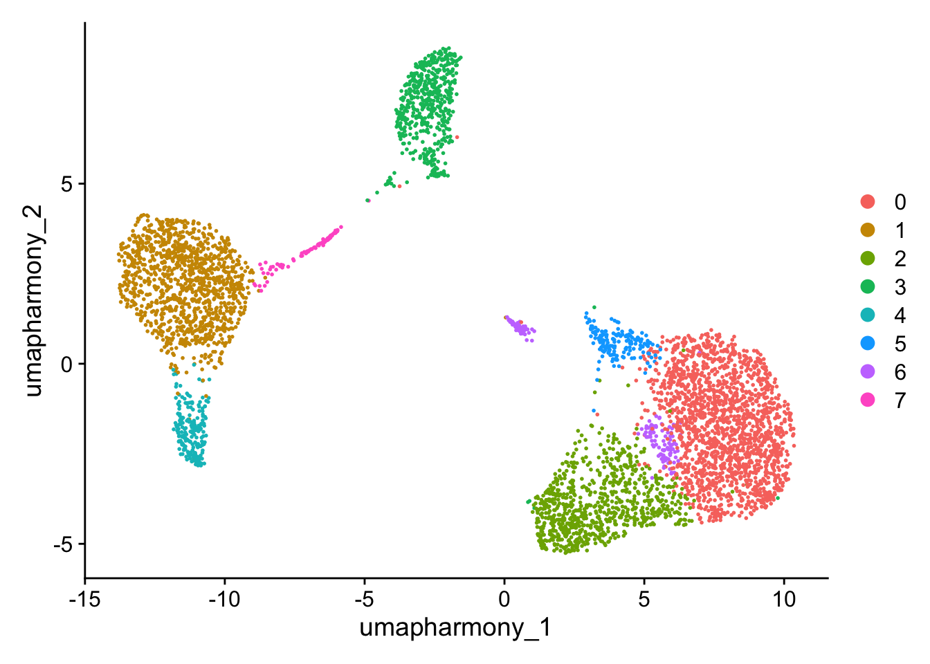
Check out the clusters.
DimPlot(seurat_object,reduction = "umap_harmony")
# Equivalent to
# DimPlot(seurat_object,reduction="umap", group.by="seurat_clusters")
# DimPlot(seurat_object,reduction="umap", group.by="RNA_snn_res.0.5")
Challenge: Try different cluster settings
Run FindNeighbours and FindClusters again, with a different number of dimensions or with a different resolution. Examine the resulting clusters using DimPlot.
To maintain the flow of this tutorial, please put the output of this exploration in a different variable, such as seurat_object2!
10.2 Choosing a cluster resolution
Its a good idea to try different resolutions when clustering to identify the variability of your data.
resolution = 2
seurat_object <- FindClusters(seurat_object, resolution = seq(0.1, resolution, 0.1))

# the different clustering created
names(seurat_object@meta.data)

# Look at cluster IDs of the first 5 cells
head(Idents(seurat_object), 5)
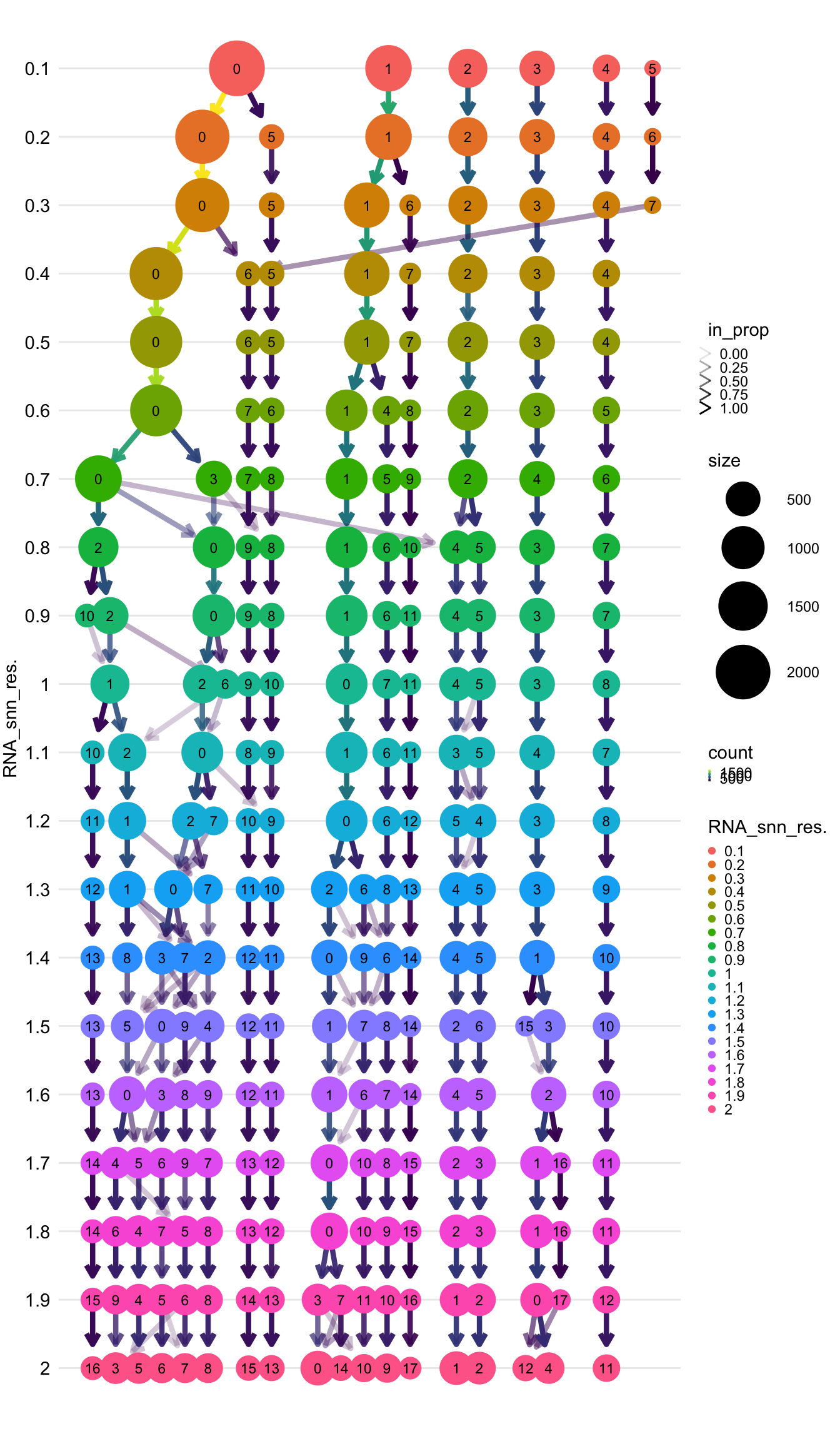
Plot a clustree to decide how many clusters you have and what resolution capture them.
library(clustree)
#> Loading required package: ggraph
#>
#> Attaching package: 'ggraph'
#> The following object is masked from 'package:sp':
#>
#>     geometry
clustree(seurat_object, prefix = "RNA_snn_res.",show_axis=TRUE) + theme(legend.key.size = unit(0.05, "cm"))
Name cells with the corresponding cluster name at the resolution you pick. This case we are happy with 0.5.
# The name of the cluster is prefixed with 'RNA_snn_res' and the number of the resolution
Idents(seurat_object) <- seurat_object$RNA_snn_res.0.5
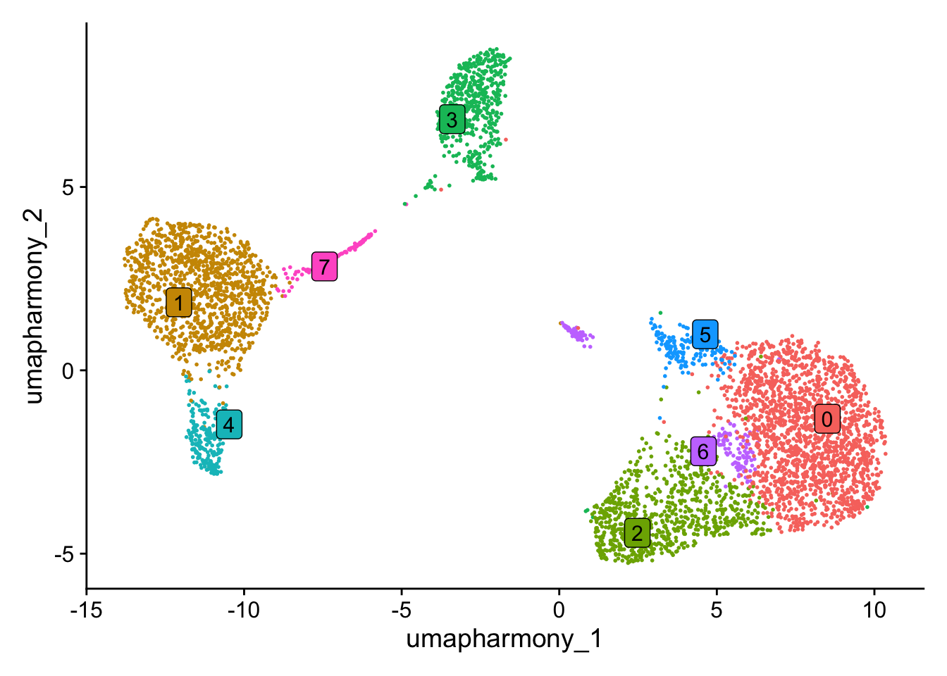
Plot the UMAP with colored clusters with Dimplot
DimPlot(seurat_object, reduction = "umap_harmony", label = TRUE, repel = TRUE, label.box = TRUE) + NoLegend()