16 ATAC Batch Correction
ATAC batch effects are assessed and corrected in this chapter using reciprocal
LSI (rLSI) integration, the chromatin-accessibility analog of the CCA strategy
applied to the RNA modality. Rather than Harmony, which operates as an
unsupervised global alignment and risks removing genuine disease-associated
chromatin variation, correction is anchor-based and directional: the merged
object is split at sample_donor resolution and the Healthy objects are used as
the integration reference, so that PASC cells are aligned onto Healthy structure
rather than the two conditions being pulled symmetrically toward each other.
Two features of ATAC data drive the choices made in this chapter. First, the peak matrix is far sparser than a gene expression matrix, so the choice of features has a much larger influence on the resulting embedding than it does for RNA; feature selection is treated as a batch correction step rather than just as preprocessing. Second, peak counts are close to binary, which changes how marker statistics behave: log fold change is maximised by rarity rather than by separation quality, so anchor features are ranked by AUC instead. Both points are developed in the sections below.
16.1 Peak-level feature selection
The features passed to RunSVD determine the coordinate system that every
downstream step inherits, so peaks are filtered before normalisation rather than
relying on a single prevalence cutoff afterwards.
Three conditions are applied jointly:
- Prevalence floor. Each peak must be detected in at least 5% of cells in every sample. This removes peaks that are effectively absent from one library.
- Cross-sample consistency. The least-detected sample must reach at least half the detection rate of the most-detected sample. This is the condition doing most of the work. A prevalence floor alone only removes peaks that are missing from a sample; a peak detected in 6% of cells in one sample and 40% in another passes a floor comfortably while acting as a near-perfect sample discriminator.
-
Global prevalence. Peaks must fall in the top quartile genome-wide. Rare
peaks are detected in only a handful of cells, so their signal is dominated by
which library happened to capture them rather than by shared biological
accessibility. This term plays the role
FindVariableFeatures()plays for RNA, curating the feature set down to broadly informative features before dimension reduction.
Peaks with zero total counts are excluded by construction, since a peak with no signal would otherwise receive a degenerate, maximal IDF weight under TF-IDF and contribute noise rather than information to the decomposition.
DefaultAssay(combined) <- "ATAC"

counts  <- GetAssayData(combined, layer = "counts")
samples <- combined$sample

detect <- sapply(unique(samples), function(s)
  Matrix::rowMeans(counts[, samples == s, drop = FALSE] > 0))

mn       <- apply(detect, 1, min)
mx       <- apply(detect, 1, max)
prev_all <- Matrix::rowMeans(counts > 0)

keep <- rownames(counts)[
  mn >= 0.05 &
  (mn / mx) >= 0.5 &
  prev_all >= quantile(prev_all, 0.75)
]

cat("Peaks retained:", length(keep), "of", nrow(counts),
    sprintf("(%.1f%%)\n", 100 * length(keep) / nrow(counts)))
#> Peaks retained: 23374 of 133851 (17.5%)
16.2 TF-IDF and LSI
TF-IDF normalisation is applied to the peak matrix and SVD is run on the filtered feature set to generate the LSI embedding.
combined <- RunTFIDF(combined)
VariableFeatures(combined) <- keep
combined <- RunSVD(combined)
16.2.1 Depth correlation
DepthCor(combined, n = 30)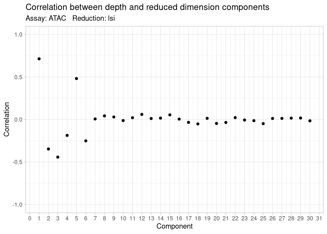
The first LSI component correlates strongly with sequencing depth and is excluded, as is standard for LSI: the leading singular vector of a TF-IDF matrix largely recovers per-cell coverage.
Components beyond the first are retained even where they show moderate depth correlation. In ATAC, total fragment count per nucleus covaries with cell type, because nuclei differ in the amount of accessible chromatin they carry. A component correlating with depth may therefore be carrying genuine cell-type identity rather than a technical artefact, and excluding such components degrades both batch mixing and cell-type resolution in this dataset. Depth is addressed at the feature level by the filtering above rather than by discarding whole components.
lsi_dims <- 2:50

combined <- RunUMAP(combined,
                    dims           = lsi_dims,
                    reduction      = "lsi",
                    reduction.name = "umap.atac",
                    reduction.key  = "atacUMAP_")
16.3 Uncorrected ATAC UMAP
Batch structure is assessed before applying any correction.
DimPlot(combined, reduction = "umap.atac", group.by = "sample") +
  ggtitle("ATAC UMAP (uncorrected) - by sample")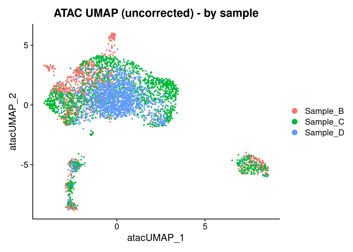
DimPlot(combined, reduction = "umap.atac", group.by = "sample_donor") +
  ggtitle("ATAC UMAP (uncorrected) - by sample-donor")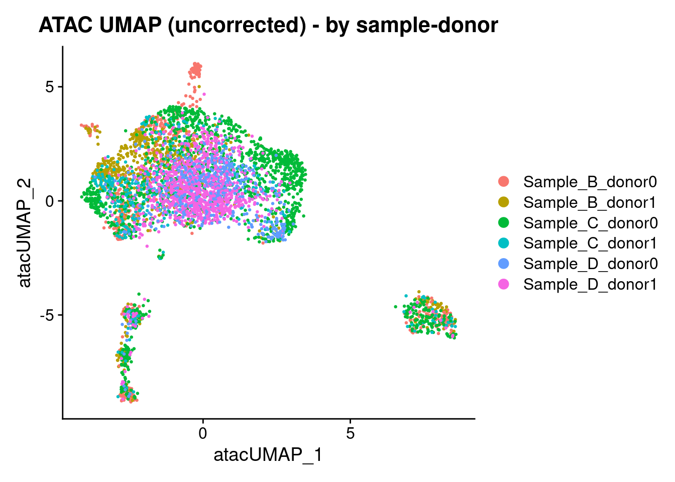
DimPlot(combined, reduction = "umap.atac", group.by = "individual_condition") +
  ggtitle("ATAC UMAP (uncorrected) - by condition")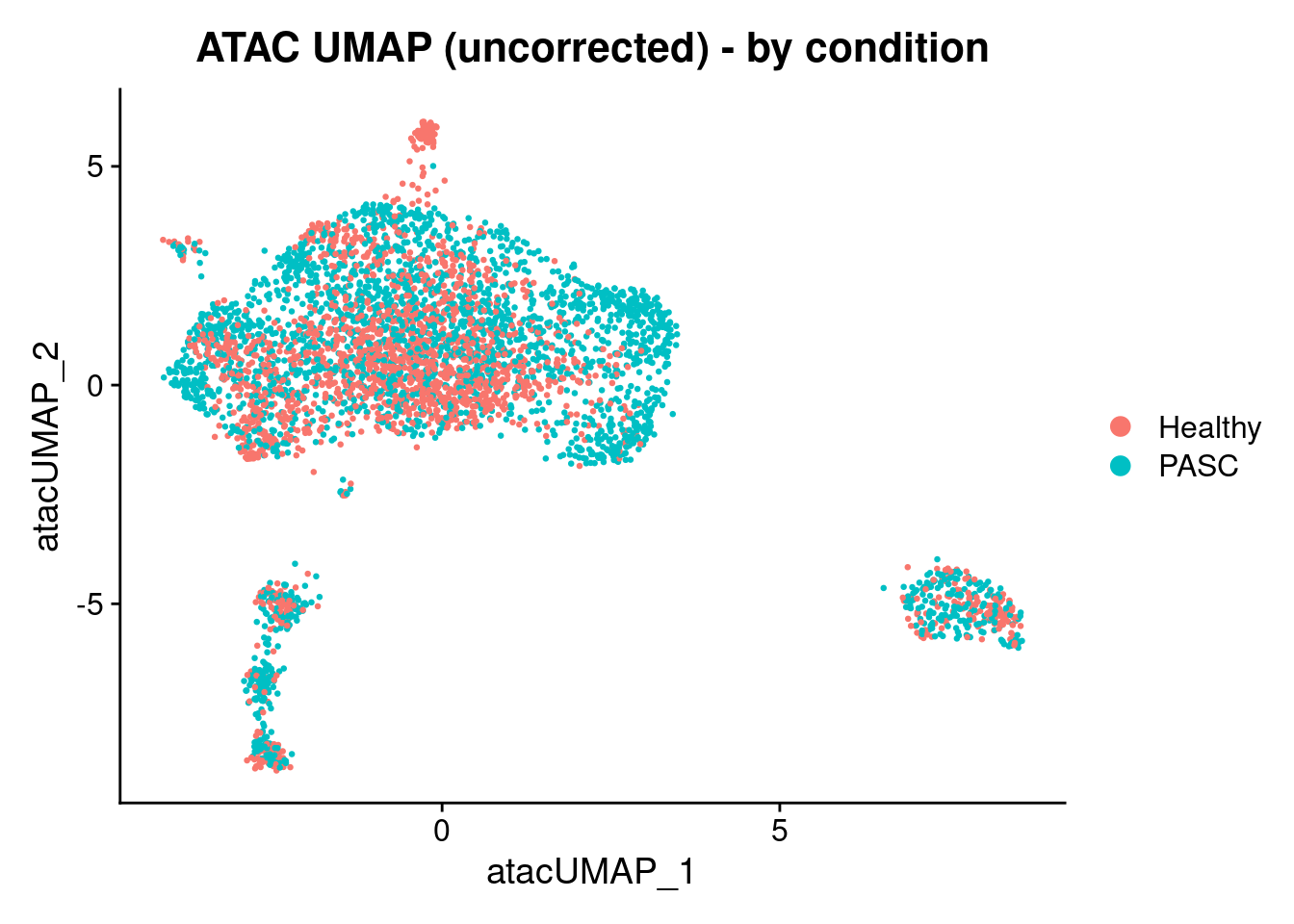
16.4 Healthy clustering
The Healthy subset is extracted and clustered to identify cell-type-defining
accessibility. Its LSI embedding is inherited from the merged object by
subsetting rows of the existing embedding rather than by re-running RunSVD on
the subset. This is a requirement rather than a convenience: reciprocal LSI
projects each object into the other’s LSI space, which is only meaningful if all
objects are rotations of the same underlying decomposition. Re-running SVD per
subset would produce independent bases and render the reciprocal projection
geometrically meaningless.
healthy_atac <- subset(combined, subset = individual_condition == "Healthy")
DefaultAssay(healthy_atac) <- "ATAC"

healthy_atac <- FindNeighbors(healthy_atac, reduction = "lsi", dims = lsi_dims)
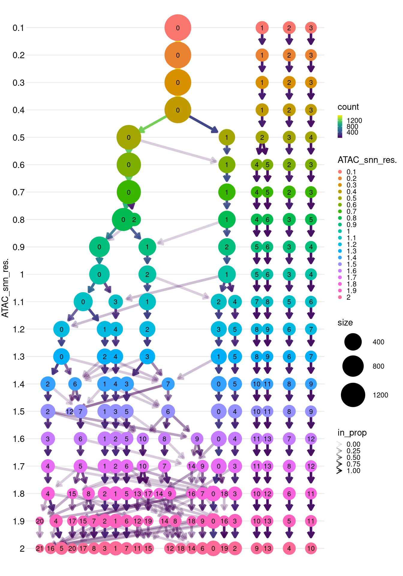
healthy_atac <- FindClusters(healthy_atac, resolution = seq(0.1, resolution, 0.1))
Idents(healthy_atac) <- healthy_atac$ATAC_snn_res.1
table(healthy_atac$ATAC_snn_res.1, healthy_atac$sample)
#>
#>     Sample_B Sample_C Sample_D
#>   0       24       33      645
#>   1      200      203       31
#>   2      113      114      205
#>   3       88       20        5
#>   4       69        0        0
#>   5       57        6        5
#>   6       25       15       15
The composition table above is a diagnostic on the clustering that defines the anchor features. A cluster dominated by a single sample indicates that the clustering has partly captured library-specific structure, which would propagate into the anchor set if left unchecked.
16.5 Anchor features
Differentially accessible peaks are identified across the Healthy clustering using a Wilcoxon test, then filtered and ranked to produce the anchor set.
Two choices differ from the equivalent RNA step and are worth stating.
Ranking by AUC rather than log fold change. On near-binary sparse data, log
fold change is maximised by rarity. A peak detected in 25% of a cluster’s cells
and 0.2% elsewhere produces a very large logFC, while a peak detected in 80%
versus 30%, a far more robust and reproducible marker, produces a modest one.
Ranking by logFC therefore selects preferentially for the sparsest peaks, which
are precisely those whose detection is most sensitive to library-specific
capture. AUC is bounded in [0, 1] and measures separation quality directly, so
it does not reward rarity in the same way.
A prevalence backbone in addition to marker peaks. One-versus-rest marker testing finds few or no discriminating peaks for populations that sit in the middle of the accessibility continuum, so a marker-only anchor set leaves those populations with almost nothing to anchor on. Adding the most broadly detected reproducible peaks gives the reciprocal projection a consistent shared frame covering all populations, including those that generate no markers of their own. These backbone peaks contribute stability rather than discrimination.
healthy_atac_markers <- wilcoxauc(
  healthy_atac,
  group_by     = "ATAC_snn_res.1",
  assay        = "data",
  seurat_assay = "ATAC"
) %>%
  tibble::as_tibble() %>%
  dplyr::filter(logFC > log(1.2) & padj < 0.01 & pct_in > 0.25)

healthy_markers_reproducible <- healthy_atac_markers %>%
  dplyr::filter(feature %in% keep)
cat("Reproducible marker peaks:", nrow(healthy_markers_reproducible),
    "of", nrow(healthy_atac_markers), "\n")
#> Reproducible marker peaks: 5923 of 33856
dplyr::count(healthy_markers_reproducible, group)
#> # A tibble: 6 × 2
#>   group     n
#>   <chr> <int>
#> 1 0        54
#> 2 1      1277
#> 3 3      2322
#> 4 4      1184
#> 5 5       810
#> 6 6       276
markers_set <- healthy_markers_reproducible %>%
  dplyr::group_by(group) %>%
  dplyr::slice_max(order_by = auc, n = 400) %>%
  dplyr::pull(feature) %>%
  unique()

prev     <- Matrix::rowMeans(counts[keep, ] > 0)
backbone <- names(sort(prev, decreasing = TRUE))[1:min(2000, length(keep))]

anchor_peaks_final <- union(markers_set, backbone)

cat("Marker-derived:", length(markers_set),
    " Backbone:", length(backbone),
    " Union:", length(anchor_peaks_final), "\n")
#> Marker-derived: 1824  Backbone: 2000  Union: 3683
The size of the anchor set matters for rLSI. Because individual peaks carry far less information than individual genes, a few hundred features are not enough to define a stable projection subspace, and anchor detection becomes unreliable exactly where populations are small or unusual. A set of several thousand peaks is appropriate here.
16.6 rLSI Integration
The merged object is split by sample_donor, giving six objects, rather than
splitting only by disease condition. Donor-level accessibility differences
within a single condition are only visible to the anchor search if each donor
has its own object to be reciprocally compared against. A two-way split pools
all Healthy donors together, leaving no way to detect or correct variation that
exists only within that pool.
The three Healthy objects are passed as reference, so anchors are found first
among the Healthy objects and each PASC object is then anchored onto that
corrected reference. Combined with anchor features derived from Healthy marker
peaks, this preserves the design intent shared with the RNA chapter:
disease-associated accessibility differences are treated as signal rather than
batch, while donor and library-level variation is treated as a confound.
IntegrateEmbeddings then corrects the full object’s LSI space using these
anchors. Unlike RNA integration, rLSI produces a corrected embedding rather than
a corrected count matrix; the original peak counts in the ATAC assay are
unchanged and remain the basis for differential accessibility testing
downstream.
atac_list <- SplitObject(combined, split.by = "sample_donor")

healthy_idx <- which(sapply(atac_list,
                     function(obj) unique(obj$individual_condition) == "Healthy"))

anchors_atac <- FindIntegrationAnchors(
  object.list     = atac_list,
  anchor.features = anchor_peaks_final,
  reduction       = "rlsi",
  reference       = healthy_idx,
  dims            = lsi_dims
)
atac_integration <- IntegrateEmbeddings(
  anchorset         = anchors_atac,
  reductions        = combined[["lsi"]],
  new.reduction     = "lsi_integration",
  dims.to.integrate = lsi_dims
)
16.7 Integrated ATAC UMAP
IntegrateEmbeddings re-indexes the integrated dimensions starting at 1. The
depth-correlated first LSI component was already excluded by passing
dims.to.integrate = lsi_dims, so it is not present in the new reduction and
there is no need to skip dimension 1 here. The number of available dimensions is
queried directly from the embedding to avoid a subscript-out-of-bounds error
when passing dims downstream.
n_integrated <- ncol(Embeddings(atac_integration, "lsi_integration"))
cat("Integrated LSI dims:", n_integrated, "\n")

atac_integration <- RunUMAP(atac_integration,
                            dims           = 1:n_integrated,
                            reduction      = "lsi_integration",
                            reduction.name = "atac.integration",
                            reduction.key  = "UMAPATACintegration_")

atac_integration <- FindNeighbors(atac_integration,
                                  reduction  = "lsi_integration",
                                  dims       = 1:n_integrated,
                                  graph.name = c("atac.integration_nn",
                                                 "atac.integration_snn"))

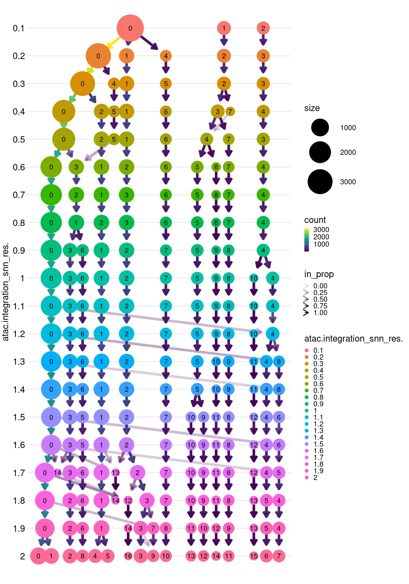
atac_integration <- FindClusters(atac_integration,
                                 graph.name = "atac.integration_snn",
                                 resolution = seq(0.1, resolution, 0.1))
DimPlot(atac_integration, reduction = "atac.integration", group.by = "sample") +
  ggtitle("ATAC UMAP (rLSI integrated) - by sample")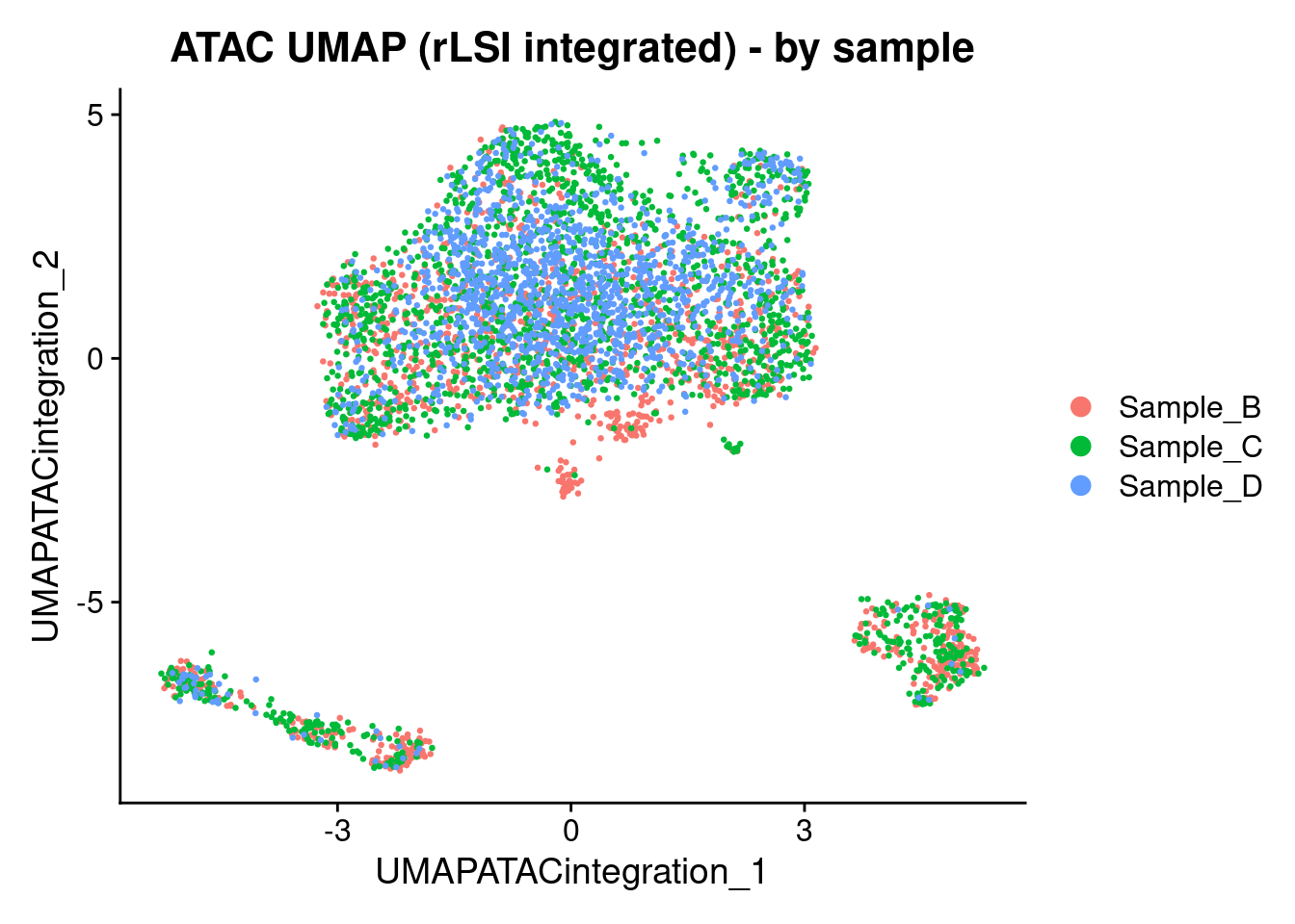
DimPlot(atac_integration, reduction = "atac.integration", group.by = "sample_donor") +
  ggtitle("ATAC UMAP (rLSI integrated) - by sample-donor")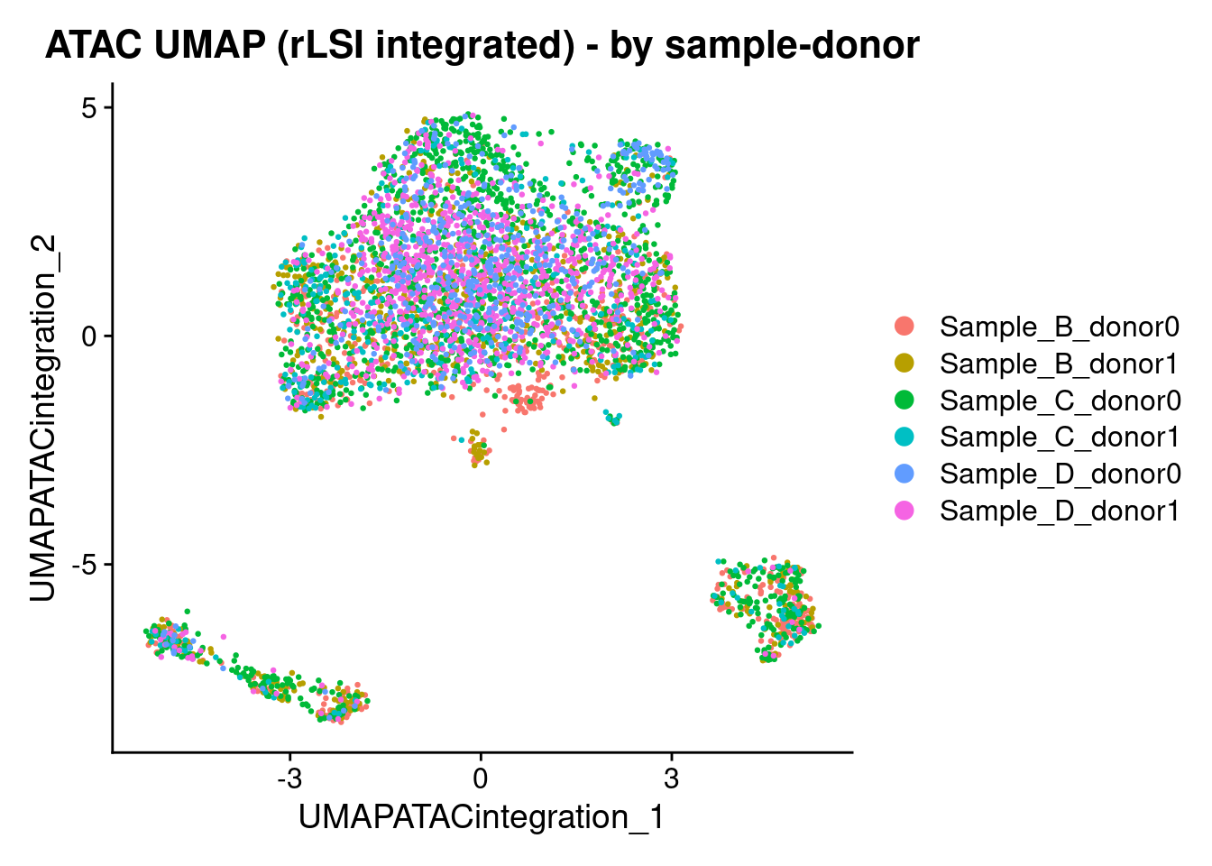
DimPlot(atac_integration, reduction = "atac.integration", group.by = "individual_condition") +
  ggtitle("ATAC UMAP (rLSI integrated) - by condition")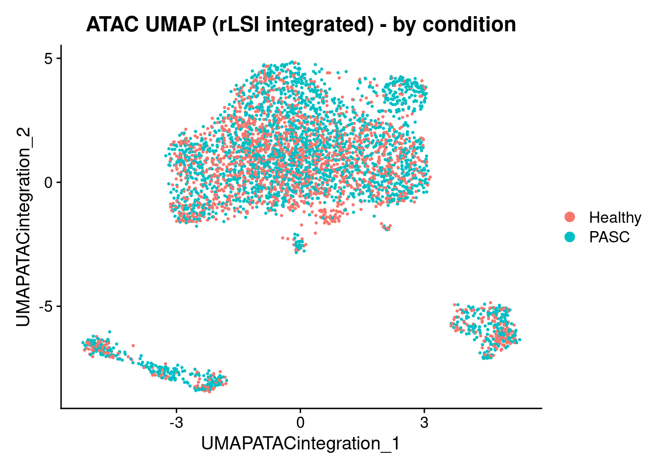
16.8 Validation
Batch correction is assessed on two criteria simultaneously, since either alone can be satisfied trivially. An embedding with no structure at all will appear perfectly mixed, and an uncorrected embedding will preserve structure while remaining unmixed.
table(atac_integration$atac.integration_snn_res.1, atac_integration$sample)
#>
#>      Sample_B Sample_C Sample_D
#>   0       400      581      799
#>   1       205      246      173
#>   2        79      325      181
#>   3       180      173      105
#>   4       134      134        6
#>   5       113       89       15
#>   6        67       96       45
#>   7        16       91       64
#>   8        55       60       27
#>   9        27        1        0
#>   10        3        8        0
table(atac_integration$atac.integration_snn_res.1, atac_integration$sample_donor)
#>
#>      Sample_B_donor0 Sample_B_donor1 Sample_C_donor0
#>   0              154             246             447
#>   1               85             120             204
#>   2               23              56             275
#>   3               76             104             107
#>   4               89              45             111
#>   5               58              55              82
#>   6               44              23              61
#>   7                4              12              77
#>   8               28              27              45
#>   9               13              14               0
#>   10               2               1               4
#>
#>      Sample_C_donor1 Sample_D_donor0 Sample_D_donor1
#>   0              134             295             504
#>   1               42              39             134
#>   2               50              70             111
#>   3               66              26              79
#>   4               23               0               6
#>   5                7               6               9
#>   6               35              13              32
#>   7               14              50              14
#>   8               15              10              17
#>   9                1               0               0
#>   10               4               0               0
The relevant signature in these tables is not uneven abundance. Cell type proportions genuinely differ between individuals, and this analysis is designed to preserve biological variation rather than flatten it. What indicates a technical artefact is a cluster with no cross-sample counterpart at all: a small population confined to a single library, typically appearing in both donors of that library, since two unrelated individuals sequenced in one lane share only the preparation.
Cell-type structure is checked against the RNA integration, which provides an independent partition of the same cells.
table(atac_integration$atac.integration_snn_res.1,
      rna_integration$rna.integration_snn_res.1)
#>
#>        0   1   2   3   4   5   6   7   8   9  10  11
#>   0  326 245 247 198 130 138 130 155  90  85  24  12
#>   1  112  74  65 132  45  57  42  25  26  30  13   3
#>   2  113  84  91  56  40  40  48  48  28  25   9   3
#>   3   67 111  47  57  47  29  35  18  23  13   8   3
#>   4   41  21  30  21  17  16   5   8  98  10   2   5
#>   5   29  22  26  21  12   9  11   6   6  18  54   3
#>   6   30  56  19  24  23  14  11   4  14   8   4   1
#>   7   15  25  13  16   8  14  30  35   7   5   2   1
#>   8   12  19  10  19   9   8   7   1   9  46   0   2
#>   9    0   8   4   2   3   1   0   3   2   1   3   1
#>   10   1   3   1   0   0   3   1   0   0   0   0   2
Correspondence between the two modalities is expected to be partial rather than one-to-one. Chromatin accessibility resolves major lineages well but has less power than the transcriptome to separate fine subsets within a lineage, so RNA clusters representing activation or memory states of the same cell type may map onto a single ATAC cluster. A loss of correspondence for major lineages, in contrast, indicates that feature filtering has removed cell-type-defining signal.
16.9 Save corrected assay
DefaultAssay(atac_integration) <- "ATAC"
SaveSeuratRds(atac_integration, "data/atac_batch_corrected.rds")
16.10 Conclusion
ATAC batch correction was performed using reciprocal LSI integration rather than
Harmony (see the dropped steps section). Harmony was evaluated but found to
overcorrect: the sample_donor grouping variable is confounded with
individual_condition, since each sample-donor combination corresponds to a
single individual with a fixed PASC or Healthy status. Correcting on that
variable removes genuine disease-associated chromatin accessibility variation
alongside technical batch effects, producing a fragmented UMAP with disconnected
clusters not present in the uncorrected embedding.
The approach taken here addresses batch effects at two levels. At the feature level, peaks are required to be detected consistently across all three samples before entering the decomposition, which removes library-specific peaks at the point where they would otherwise define the coordinate system. At the anchor level, integration is performed across all six sample-donor objects with the Healthy objects as reference, using AUC-ranked marker peaks supplemented by a prevalence backbone, so that donor-level variation is corrected while disease-associated variation is preserved as signal.
Feature selection proved to be the dominant control on batch structure in this modality, more so than either the choice of retained LSI dimensions or the size of the anchor set. This reflects the sparsity of the peak matrix: a peak detected in a small number of cells carries little biological information but can strongly influence the decomposition, and whether it is detected at all depends substantially on library preparation. Filtering on cross-sample reproducibility targets that mechanism directly, rather than removing sparse peaks indiscriminately and losing genuine signal alongside them.
The corrected embedding (lsi_integration) feeds into the weighted
nearest-neighbour graph in the cross-modal integration chapter. Differential
accessibility testing in downstream chapters uses the original ATAC assay
counts, which are unmodified by rLSI.