30 Trajectory Analysis (Monocle3)
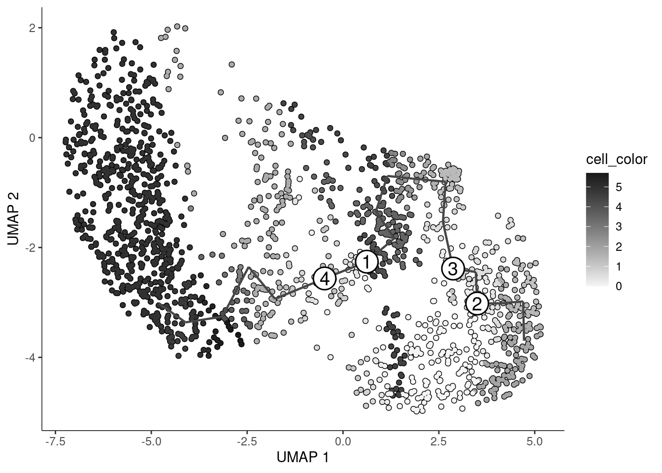
Monocle3 orders cells along a learned principal graph (pseudotime) rooted
at a chosen starting cluster, visualising differentiation-like structure as
a single branching tree over the WNN embedding. cluster_6 is used as the
root, as in the original analysis; clusters 6 and 7 are excluded before
learning the trajectory, also matching the original analysis. The
trajectory is learned once on the full dataset, and again separately on the
PASC-only and Healthy-only subsets, to compare pseudotime progression and
branch usage between the two conditions on a matched cluster structure.
30.1 Load object and build a 3D companion embedding
A 3D UMAP is computed alongside the existing 2D integration.wnn embedding
from the same weighted nearest-neighbour graph, for the 3D trajectory view
further down.
library(SeuratWrappers)
library(monocle3)
library(ggplot2)
library(dplyr)
library(tidyr)
set.seed(1234)
combined@assays[["regulon"]]@key <- "regulon_"
combined <- RunUMAP(combined, nn.name = "weighted.nn", assay = "RNA",
                    reduction.name = "integration.wnn.3d", n.components = 3)

# this was with the first run of the object
combined <- combined[, !combined$cell_labels %in% c("cluster_5", "cluster_7", "cluster_8")]
30.2 Build trajectory helper
as.cell_data_set() embeds Seurat reductions into the monocle
cell_data_set by copying whatever reducedDims slots the intermediate
SingleCellExperiment coercion produced. The original script relied on
those slots’ numeric position (reducedDims(sce)[[5]],
reducedDims(sce)[[6]], …), which is fragile and breaks silently if
Seurat’s internal reduction ordering changes; the UMAP embeddings needed
for cluster_cells()/learn_graph() are assigned directly by name
instead.
build_trajectory <- function(obj, root_cluster = "cluster_6") {
  cds <- as.cell_data_set(obj, assay = "RNA")

  umap2d <- Embeddings(obj, "integration.wnn")[colnames(cds), , drop = FALSE]
  umap3d <- Embeddings(obj, "integration.wnn.3d")[colnames(cds), , drop = FALSE]

  reducedDim(cds, "UMAP")   <- umap2d
  reducedDim(cds, "UMAP3D") <- umap3d

  root_cells <- colnames(obj)[obj$cell_labels == root_cluster]

  cds <- cluster_cells(cds, reduction_method = "UMAP")
  cds <- learn_graph(cds, use_partition = TRUE)
  cds <- order_cells(cds, reduction_method = "UMAP", root_cells = root_cells)
  cds
}

build_trajectory_3d <- function(obj, root_cluster = "cluster_6") {
  cds <- as.cell_data_set(obj, assay = "RNA")

  umap3d <- Embeddings(obj, "integration.wnn.3d")[colnames(cds), , drop = FALSE]
  reducedDim(cds, "UMAP") <- umap3d   # must be literally "UMAP" for plot_cells_3d

  root_cells <- colnames(obj)[obj$cell_labels == root_cluster]

  cds <- cluster_cells(cds, reduction_method = "UMAP")
  cds <- learn_graph(cds, use_partition = TRUE)
  cds <- order_cells(cds, reduction_method = "UMAP", root_cells = root_cells)
  cds
}

summarise_trajectory <- function(cds) {
  pseudo_df <- data.frame(
    celllabels = cds$cell_labels,
    condition  = cds$individual_condition,
    pseudo     = pseudotime(cds)
  )

  print(
    pseudo_df %>%
      group_by(celllabels, condition) %>%
      summarise(mean_pseudo = mean(pseudo, na.rm = TRUE), .groups = "drop")
  )

 print(
  ggplot(pseudo_df, aes(x = celllabels, y = pseudo, fill = condition)) +
    geom_boxplot() +
    theme(axis.text.x = element_text(angle = 90, hjust = 1, vjust = 0.5))
)

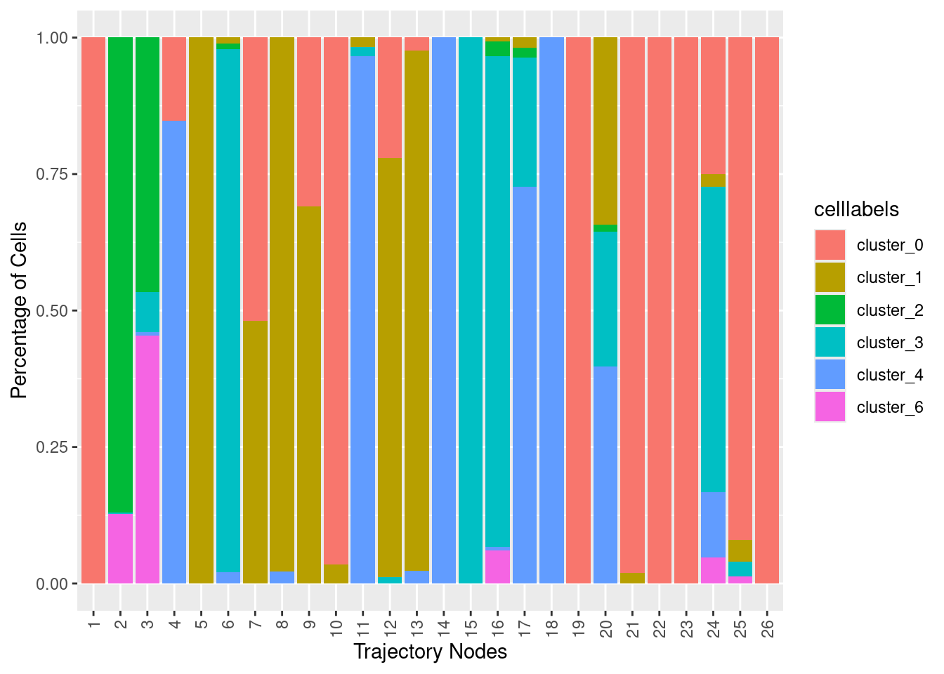
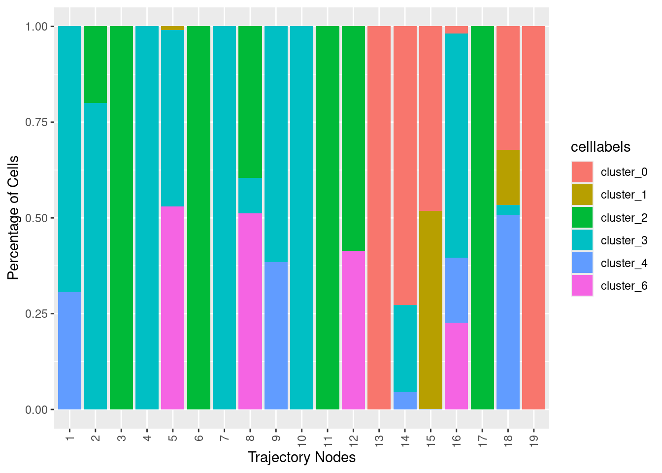
  closest_vertex <- cds@principal_graph_aux[["UMAP"]]$pr_graph_cell_proj_closest_vertex
  count_node_df <- data.frame(table(data.frame(
    celllabels = cds$cell_labels,
    condition  = cds$individual_condition,
    node       = as.matrix(closest_vertex[colnames(cds), ])
  )))

  print(
    ggplot(count_node_df, aes(y = Freq, x = node, fill = celllabels)) +
      geom_bar(position = "fill", stat = "identity") +
      xlab("Trajectory Nodes") + ylab("Percentage of Cells")+
          theme(axis.text.x = element_text(angle = 90, hjust = 1, vjust = 0.5))

  )

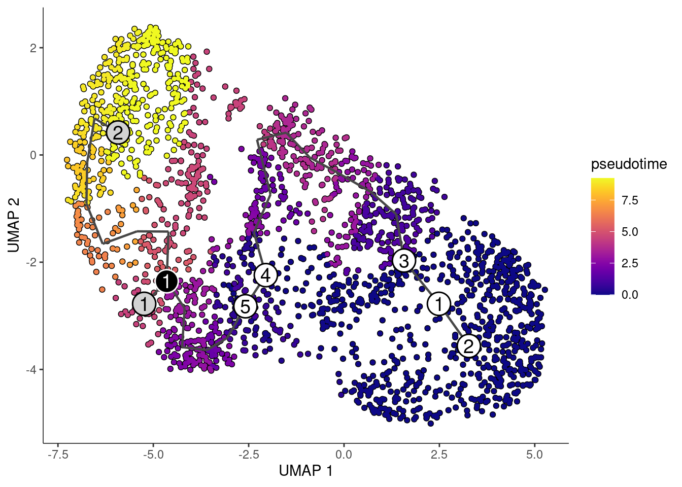
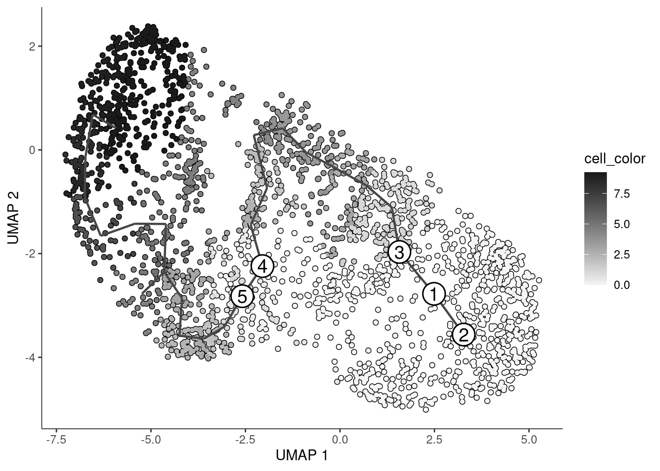
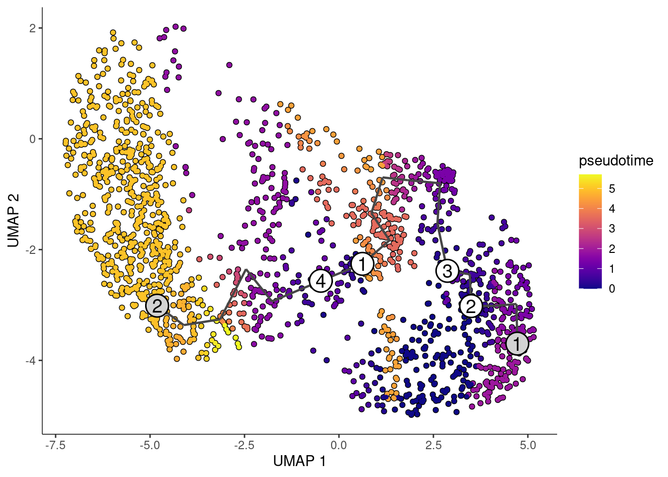
  print(
    plot_cells(cds, color_cells_by = "pseudotime", show_trajectory_graph = TRUE,
              cell_size = 1, trajectory_graph_segment_size = 0.8, graph_label_size = 5)
  )

  print(
    plot_cells(cds, color_cells_by = "pseudotime", show_trajectory_graph = TRUE,
              cell_size = 1, trajectory_graph_segment_size = 0.8, graph_label_size = 5,
              label_leaves = FALSE, label_branch_points = FALSE) +
      scale_colour_gradient(low = "grey96", high = "grey10")
  )
}
30.3 Full dataset
cds_all <- build_trajectory(combined)
#>   |                                                          |                                                  |   0%  |                                                          |==================================================| 100%
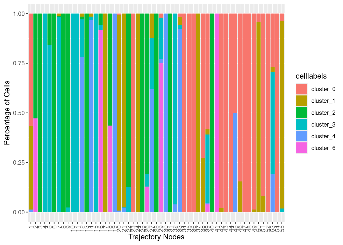
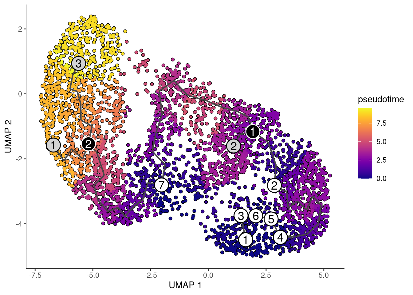
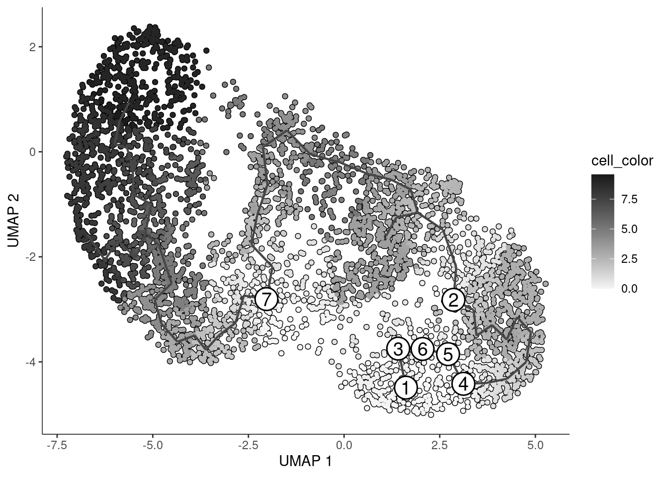
summarise_trajectory(cds_all)
#> # A tibble: 12 × 3
#>    celllabels condition mean_pseudo
#>    <chr>      <chr>           <dbl>
#>  1 cluster_0  Healthy         4.32
#>  2 cluster_0  PASC            3.42
#>  3 cluster_1  Healthy         7.83
#>  4 cluster_1  PASC            8.14
#>  5 cluster_2  Healthy         1.85
#>  6 cluster_2  PASC            1.92
#>  7 cluster_3  Healthy         2.72
#>  8 cluster_3  PASC            2.86
#>  9 cluster_4  Healthy         3.72
#> 10 cluster_4  PASC            3.86
#> 11 cluster_6  Healthy         0.185
#> 12 cluster_6  PASC            0.135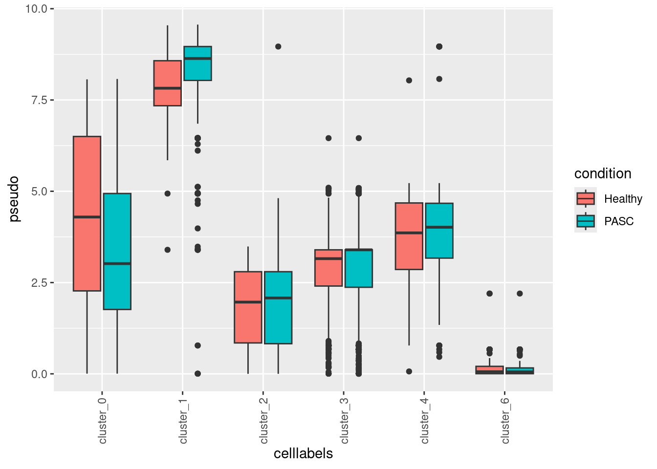
30.3.1 Top markers by cell type
marker_test_res <- top_markers(cds_all, group_cells_by = "cell_labels",
                               reference_cells = 1000, cores = 8)

top_specific_marker_ids <- marker_test_res %>%
  dplyr::filter(fraction_expressing >= 0.10) %>%
  group_by(cell_group) %>%
  top_n(1, pseudo_R2) %>%
  pull(gene_id) %>%
  unique()

rowData(cds_all)$gene_short_name <- row.names(rowData(cds_all))
plot_genes_by_group(cds_all, top_specific_marker_ids, group_cells_by = "cell_labels",
                    ordering_type = "maximal_on_diag", max.size = 3)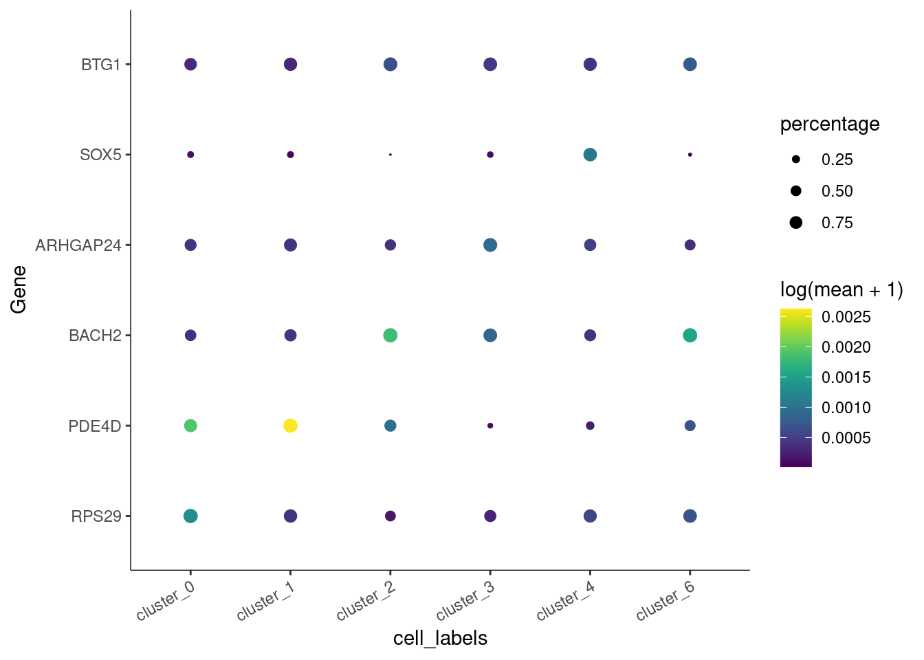
30.3.2 3D trajectory
cds_all_3d <- build_trajectory_3d(combined)
#>   |                                                          |                                                  |   0%  |                                                          |==================================================| 100%
plot_cells_3d(cds_all_3d, reduction_method = "UMAP", color_cells_by = "pseudotime")
30.4 PASC only
cds_pasc <- build_trajectory(combined[, combined$individual_condition == "PASC"])
#>   |                                                          |                                                  |   0%  |                                                          |==================================================| 100%
summarise_trajectory(cds_pasc)
#> # A tibble: 6 × 3
#>   celllabels condition mean_pseudo
#>   <chr>      <chr>           <dbl>
#> 1 cluster_0  PASC           2.94
#> 2 cluster_1  PASC           8.03
#> 3 cluster_2  PASC           0.0325
#> 4 cluster_3  PASC           1.11
#> 5 cluster_4  PASC           2.95
#> 6 cluster_6  PASC           0.0198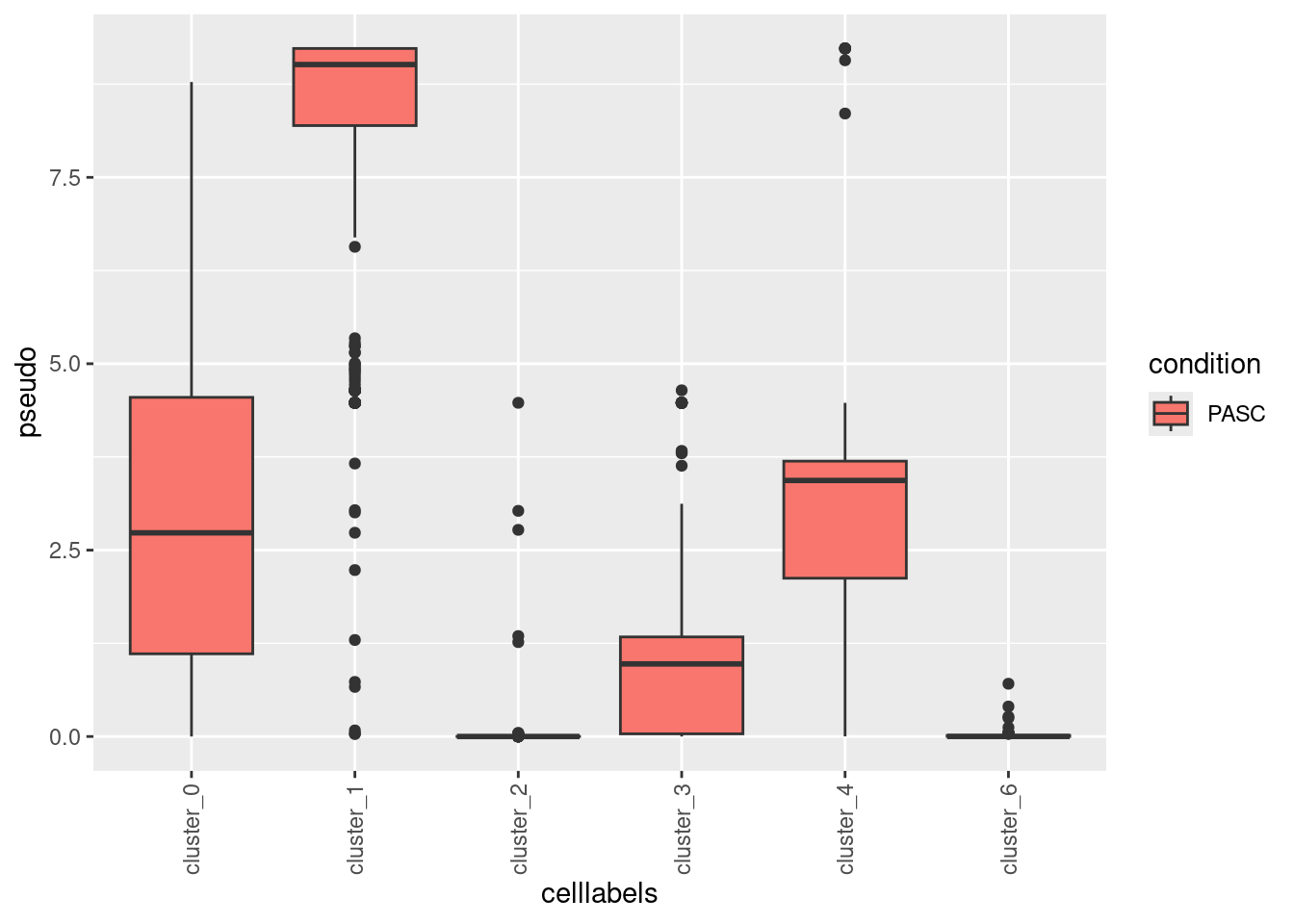
30.5 Healthy only
cds_healthy <- build_trajectory(combined[, combined$individual_condition == "Healthy"])
#>   |                                                          |                                                  |   0%  |                                                          |==================================================| 100%
summarise_trajectory(cds_healthy)
#> # A tibble: 6 × 3
#>   celllabels condition mean_pseudo
#>   <chr>      <chr>           <dbl>
#> 1 cluster_0  Healthy         4.41
#> 2 cluster_1  Healthy         4.78
#> 3 cluster_2  Healthy         0.982
#> 4 cluster_3  Healthy         2.41
#> 5 cluster_4  Healthy         2.40
#> 6 cluster_6  Healthy         1.05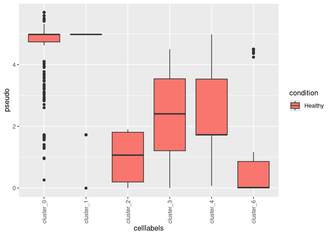
30.6 Export trajectory graph for ShinyCellModular
The per-cell pseudotime values saved above are ordinary numeric columns, but
the branching structure learn_graph() fitted is not a per-cell value, it is
a small graph between principal-graph nodes. It has no natural home in
meta.data, so it is stored in combined@misc$trajectory_graph instead,
keyed by the same column names used for pseudotime, so the app can match them
up. cds_all supplies the 2D graph and cds_all_3d the 3D one, PASC and
Healthy were only fit in 2D in this chapter, so their dim3 entry stays
NULL
# reshape a monocle3 principal graph into a flat source/target edge table,
# for plotting only, no recalculation. reads the graph learn_graph() already
# built for the given reduction


extract_monocle_edges <- function(cds, reduction = "UMAP") {
  dp_mst <- cds@principal_graph[[reduction]]
  if (is.null(dp_mst)) stop("No principal graph for reduction '", reduction, "'", call. = FALSE)

  raw <- cds@principal_graph_aux[[reduction]]$dp_mst
  ndim <- nrow(raw)
  coords <- as.data.frame(t(raw))
  colnames(coords) <- c("x", "y", "z")[seq_len(ndim)]
  coords$node <- rownames(coords)

  edges <- as.data.frame(igraph::as_edgelist(dp_mst), stringsAsFactors = FALSE)
  colnames(edges) <- c("from", "to")
  edges <- merge(edges, coords, by.x = "from", by.y = "node")
  edges <- merge(edges, coords, by.x = "to", by.y = "node", suffixes = c("_source", "_target"))
  edges[, grep("_source$|_target$", colnames(edges))]
}


combined@misc$trajectory_graph <- c(
  combined@misc$trajectory_graph,
  list(
    pseudotime_all     = list(dim2 = extract_monocle_edges(cds_all),     dim3 = extract_monocle_edges(cds_all_3d)),
    pseudotime_pasc    = list(dim2 = extract_monocle_edges(cds_pasc),    dim3 = NULL),
    pseudotime_healthy = list(dim2 = extract_monocle_edges(cds_healthy), dim3 = NULL)
  )
)
30.7 Save results
combined$pseudotime_all <- NA
combined$pseudotime_all[colnames(cds_all)] <- pseudotime(cds_all)

combined$pseudotime_pasc <- NA
combined$pseudotime_pasc[colnames(cds_pasc)] <- pseudotime(cds_pasc)

combined$pseudotime_healthy <- NA
combined$pseudotime_healthy[colnames(cds_healthy)] <- pseudotime(cds_healthy)
SaveSeuratRds(combined, "data/seurat_object_cross_modal_integration_peakslinks_motifs_grn_regulons_monoclepseudotime.rds")

saveRDS(
  list(cds_all = cds_all, cds_pasc = cds_pasc, cds_healthy = cds_healthy,
       marker_test_res = marker_test_res, top_specific_marker_ids = top_specific_marker_ids),
  "data/monocle3_trajectory_results.rds"
)