28 Condition-Specific GRN Visualisation

Pando’s own graph utilities (get_network_graph, plot_network_graph, get_tf_network, plot_tf_network) are used here to visualise regulatory subnetworks around a small set of TFs of interest — one set associated with PASC, one with Healthy — extracted from the combined GRN built in the Gene Regulatory Network Inference chapter. The next chapter (TF Regulatory Subnetwork Diagrams) revisits the same TF sets with a lighter-weight, ggraph-only alternative built directly from the regulon-to-target table, without depending on Pando’s graph objects.

28.1 TF sets of interest and their regulon targets

library(dplyr)

TF_regulation <- read.table("data/TF_regulation.txt", header = TRUE)

TF_regulation %>%
  DT::datatable(extensions = "Buttons",
               options = list(dom = "Bfrtip", buttons = c("excel", "csv")))

28.2 Selected TFs

tf_PASC <- c("ARID3A", "ETS1", "ARID5B", "ZFPM1", "EGR1")
tf_healthy <- c("NR4A3", "FOXP1", "BACH2", "NFIC")

# FIXED: the original filtered on `TF$item` (the target genes) rather than
# `TF$group` (the TF/regulon itself), which would return targets of
# already-selected targets instead of the TFs' own target genes.
features_PASC <- TF_regulation$item[TF_regulation$group %in% tf_PASC]
features_healthy <- TF_regulation$item[TF_regulation$group %in% tf_healthy]

28.3 PASC subnetwork

grn_object_PASC <- get_network_graph(grn_object,
                                     graph_name = "sub_graph",
                                     umap_method = "none",
                                     features = c(tf_PASC, features_PASC))

plot_network_graph(grn_object_PASC, graph = "sub_graph", layout = "drl",
                   color_nodes = TRUE, node_size = 5)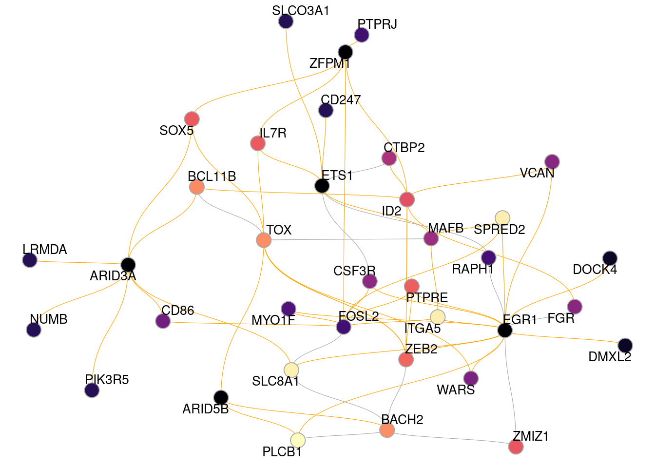

Download PDF

grn_object_tf_PASC <- get_tf_network(grn_object_PASC,
                                     tf = "ARID5B",
                                     features = c(tf_PASC, features_PASC),
                                     graph = "sub_graph",
                                     keep_all_edges = TRUE)

plot_tf_network(grn_object_tf_PASC, tf = "ARID5B", circular = TRUE)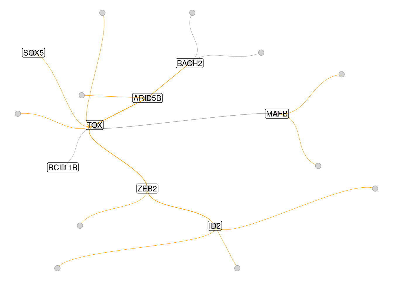

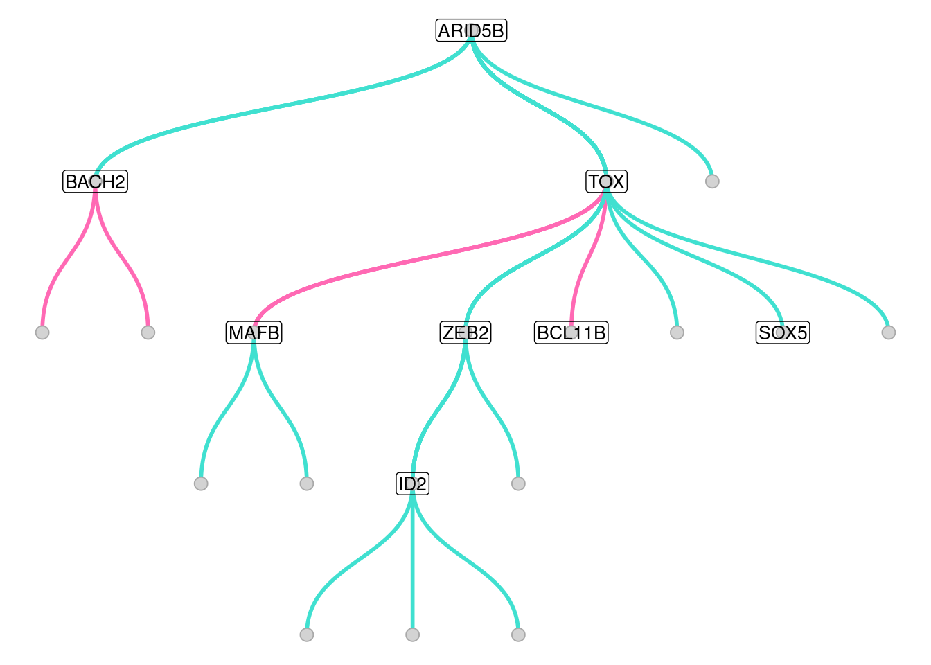
Download PDF

plot_tf_network(
  grn_object_tf_PASC,
  tf = "ARID5B",
  edge_color = c("hotpink", "turquoise"),
  circular = FALSE,
  edge_width = 1
)

Download PDF

28.4 Healthy subnetwork

grn_object_healthy <- get_network_graph(grn_object,
                                        graph_name = "sub_graph",
                                        umap_method = "none",
                                        features = c(tf_healthy, features_healthy))

grn_object_healthy <- get_tf_network(grn_object_healthy,
                                     tf = "BACH2",
                                     features = c(tf_healthy, features_healthy),
                                     graph = "sub_graph",
                                     keep_all_edges = TRUE)

plot_tf_network(grn_object_healthy, tf = "BACH2", circular = TRUE)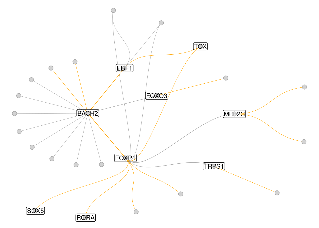

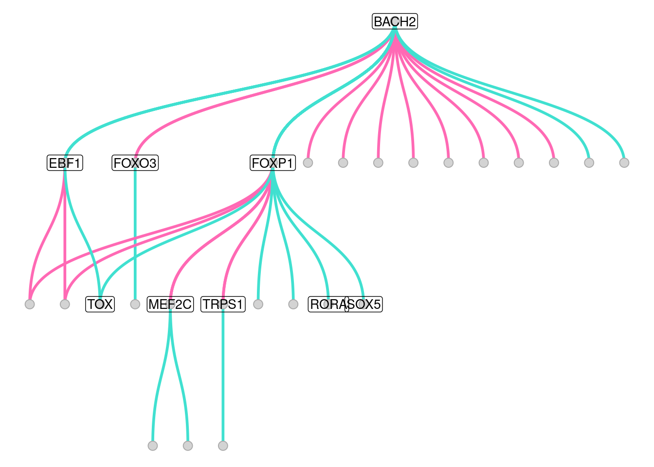
Download PDF

plot_tf_network(
  grn_object_healthy,
  tf = "BACH2",
  edge_color = c("hotpink", "turquoise"),
  circular = FALSE,
  edge_width = 1
)

Download PDF

28.5 Combined subnetwork

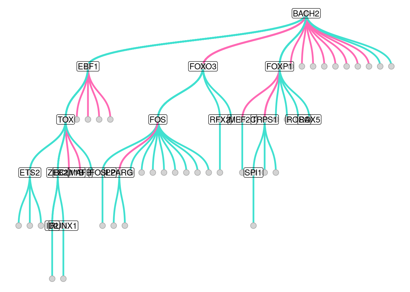
Both TF sets are shown together on the full network, centred on BACH2, to compare how the PASC- and Healthy-associated TFs relate to one another rather than viewing each in isolation.

# FIXED: `data/grn_object.rds` (Gene Regulatory Network Inference chapter) was
# saved before its "full_graph" was computed — that chapter assigns
# get_network_graph()'s result to a separate `grn_object_network` variable and
# saves the original `grn_object` instead, so `graph = "full_graph"` below
# would otherwise fail with "The requested graph 'full_graph' does not exist."
grn_object <- get_network_graph(grn_object, graph_name = 'full_graph', umap_method = 'none')

grn_object_combined <- get_tf_network(grn_object,
                                      tf = "BACH2",
                                      features = c(tf_healthy, features_healthy,
                                                  tf_PASC, features_PASC),
                                      graph = "full_graph")

plot_tf_network(grn_object_combined, tf = "BACH2", circular = FALSE)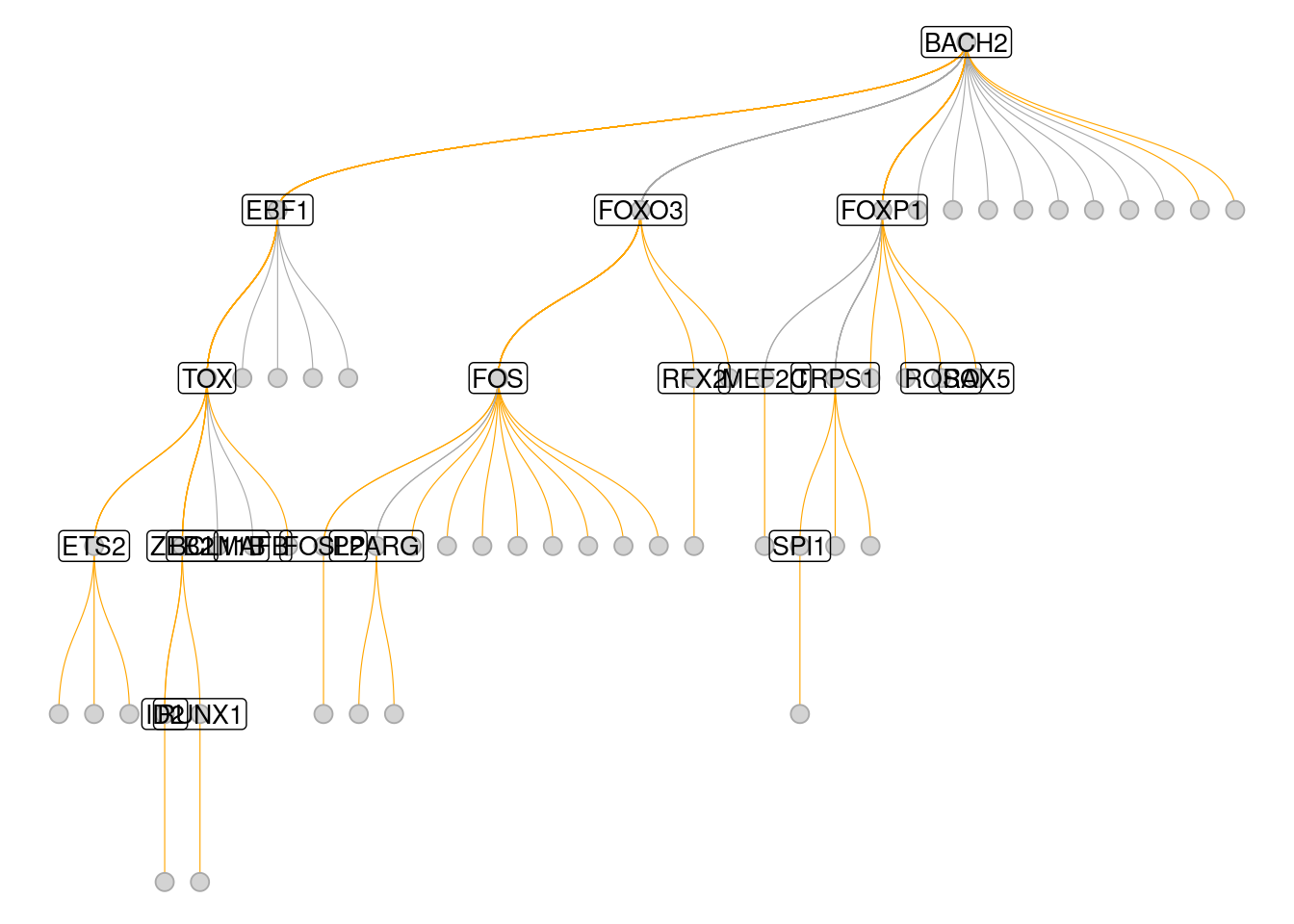

Download PDF

plot_tf_network(
  grn_object_combined,
  tf = "BACH2",
  edge_color = c("hotpink", "turquoise"),
  circular = FALSE,
  edge_width = 1
)

Download PDF