23 Gene Regulatory Network Inference
Pando infers a gene regulatory network (GRN) by combining TF motif matches in ATAC peaks with a linear model of gene expression as a function of (a) the expression of TFs with a predicted binding site near the gene and (b) the accessibility of the peak containing that binding site. This makes the network condition- and accessibility-aware, rather than relying on TF-gene co-expression alone. Networks are built separately for the PASC and Healthy conditions to allow the resulting regulons to be compared between condition, and once on the full object to identify the overall set of significant TF-peak-target trios used for regulon module detection.
23.1 Load object and marker genes
library(Seurat)
library(Signac)
library(Pando)
library(doParallel)
library(dplyr)
library(arrow)
library(BSgenome.Hsapiens.UCSC.hg38)
library(doParallel)

markers_genes_list_roc <- open_dataset("data/markers_genes_list_wsnn_all_resolutions.parquet")

grn_candidate_genes <- markers_genes_list_roc %>%
   dplyr::filter(annotation == "wsnn_res.0.5") %>%  dplyr::filter(auc > 0.7) %>% dplyr::select("feature") %>%
  collect()

grn_candidate_genes <- grn_candidate_genes$feature
registerDoParallel(20)
23.2 Combined network (all cells)
The combined-object network is used to identify the overall set of
significant TF-peak-target trios and downstream regulons, without splitting
by condition. peak_to_gene_method = "Signac" is used here (rather than
"GREAT" used for the per-condition networks above) to link peaks to genes
using Signac’s distance-based linking instead of GREAT’s regulatory-domain
model.
grn <- initiate_grn(combined,
                    regions = phastConsElements20Mammals.UCSC.hg38,
                    rna_assay = "RNA", peak_assay = "ATAC")

grn <- find_motifs(grn,
                   pfm = Pando::motifs,
                   motif_tfs = Pando::motif2tf,
                   genome = BSgenome.Hsapiens.UCSC.hg38)

grn <- infer_grn(grn,
                 genes = grn_candidate_genes,
                 peak_to_gene_method = "Signac",
                 parallel = TRUE,
                 tf_cor = 0.05,
                 method = "glm",
                 family = "gaussian",
                 scale = FALSE,
                 verbose = TRUE)

coef_grn <- coef(grn) %>%  dplyr::filter(padj < 0.01)

write.table(coef_grn, "data/coef_grn.txt")
23.3 Find regulons (network modules)
library(tidyr)

grn_object <- find_modules(grn, p_thresh = 0.05, min_genes_per_module = 2)
grn_object_network <- get_network_graph(grn_object)

plot_module_metrics(grn_object_network)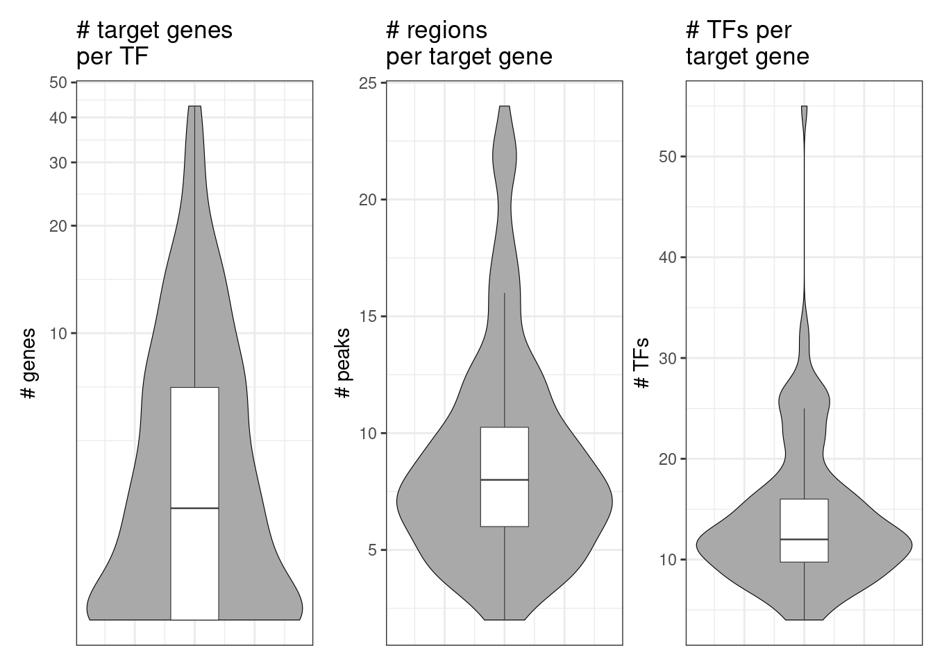
plot_gof(grn_object_network, point_size = 3)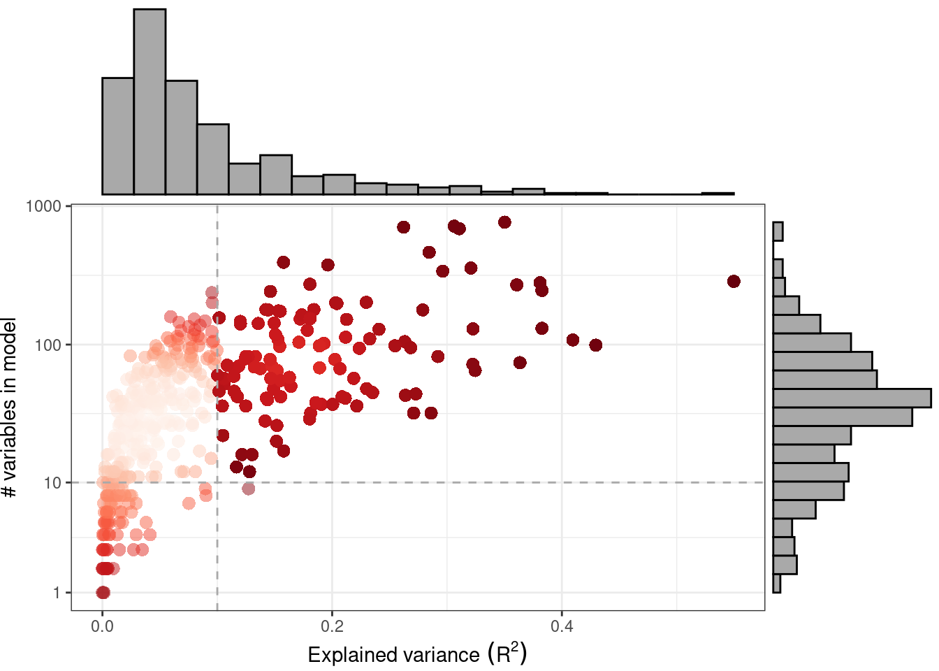
plot_network_graph(grn_object_network)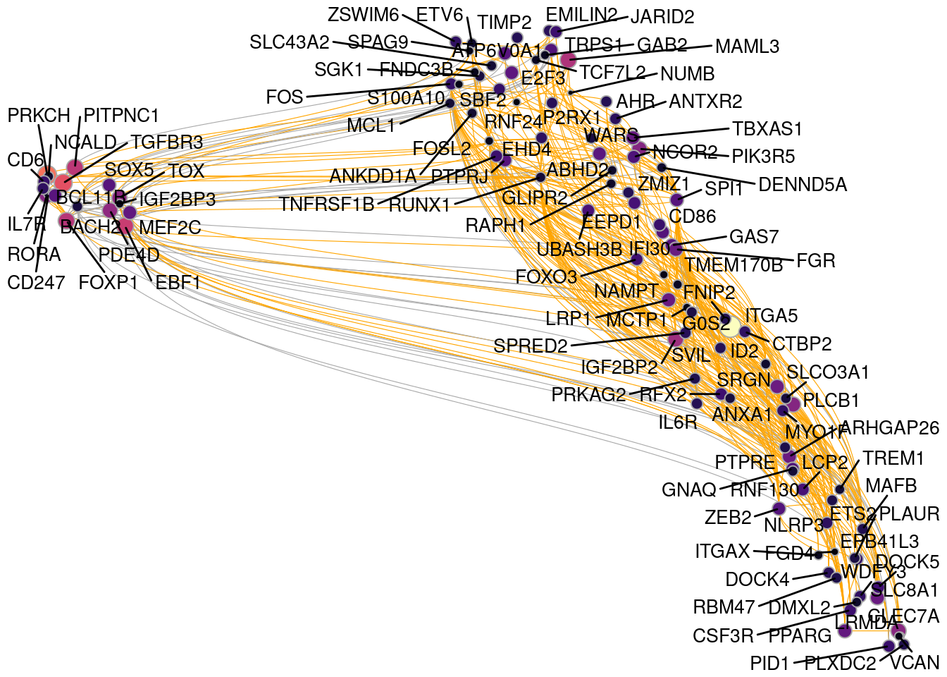
estimate is the linear model coefficient fit by Pando for a given TF-peak-gene
trio, reflecting the strength and direction of the regulatory interaction.
correlation is the global Pearson correlation between TF and target gene
expression — usually, but not necessarily, the same sign as estimate, since
the linear model accounts for additional terms. statistic is the test
statistic underlying the coefficient’s p-value; its exact form depends on
the model-fitting method used.
regulons <- NetworkModules(grn_object)
regulons@meta
#> # A tibble: 1,582 × 9
#>    tf     target estimate n_regions n_genes n_tfs regions
#>    <chr>  <chr>     <dbl>     <int>   <int> <int> <chr>
#>  1 ADNP   MEF2C     0.129        12       1    12 chr5-8883…
#>  2 AEBP2  ZSWIM6    0.101         6       1     8 chr5-6133…
#>  3 AHRR   LRP1      0.237        22       1    27 chr12-570…
#>  4 ARID3A BCL11B    0.442        19       7    26 chr14-992…
#>  5 ARID3A CD86      0.225        13       7    16 chr3-1220…
#>  6 ARID3A LRMDA     0.134        22       7    55 chr10-764…
#>  7 ARID3A NUMB      0.109         6       7     7 chr14-733…
#>  8 ARID3A PIK3R5    0.122        10       7    17 chr17-880…
#>  9 ARID3A SLC8A1    0.341        14       7    26 chr2-4047…
#> 10 ARID3A SOX5      0.184        17       7    18 chr12-239…
#> # ℹ 1,572 more rows
#> # ℹ 2 more variables: pval <dbl>, padj <dbl>

write.table(regulons@meta, "data/regulones.txt", row.names = FALSE)
23.4 Subnetwork visualisation
A subnetwork can be extracted around a set of TFs of interest for focused visualisation, e.g. the immediate-early / AP-1 family TFs below.
grn_object_subset <- get_network_graph(
  grn_object,
  graph_name = "sub_graph",
  umap_method = "none",
  features = c("BCL6", "CCDC88A", "CREB3L2", "EGR1", "ELF1", "ETS2", "ETV6",
              "FOS", "FOSB", "FOSL1", "FOSL2", "FOXO1", "GATAD2A")
)

plot_network_graph(grn_object_subset, graph = "sub_graph", layout = "fr",
                   color_nodes = FALSE, node_size = 5)


grn_object_tf <- get_tf_network(grn_object, tf = "MEF2A")
plot_tf_network(grn_object_tf, tf = "MEF2A")
plot_tf_network(grn_object_tf, circular = FALSE)
23.5 Save GRN-annotated object
The Seurat object itself is unchanged by GRN inference (Pando stores the
network separately), but is re-saved under a new name to mark this stage of
the pipeline. The grn_object (containing the regulon modules used in the
next chapter) is saved separately, since it is not part of the Seurat object
and would otherwise only exist in this chapter’s in-memory session.
SaveSeuratRds(combined, "data/seurat_object_cross_modal_integration_peakslinks_motifs_grn.rds")
saveRDS(grn_object, "data/grn_object.rds")